
速度二次规划优化算法主要是执行PIECEWISE_JERK_SPEED task,然后PiecewiseJerkSpeedOptimizer::Process会被调用
Status PiecewiseJerkSpeedOptimizer::Process(const PathData& path_data,
                                            const TrajectoryPoint& init_point,
                                            SpeedData* const speed_data)
std::array<double, 3> init_s = {0.0, st_graph_data.init_point().v(),
                                st_graph_data.init_point().a()};
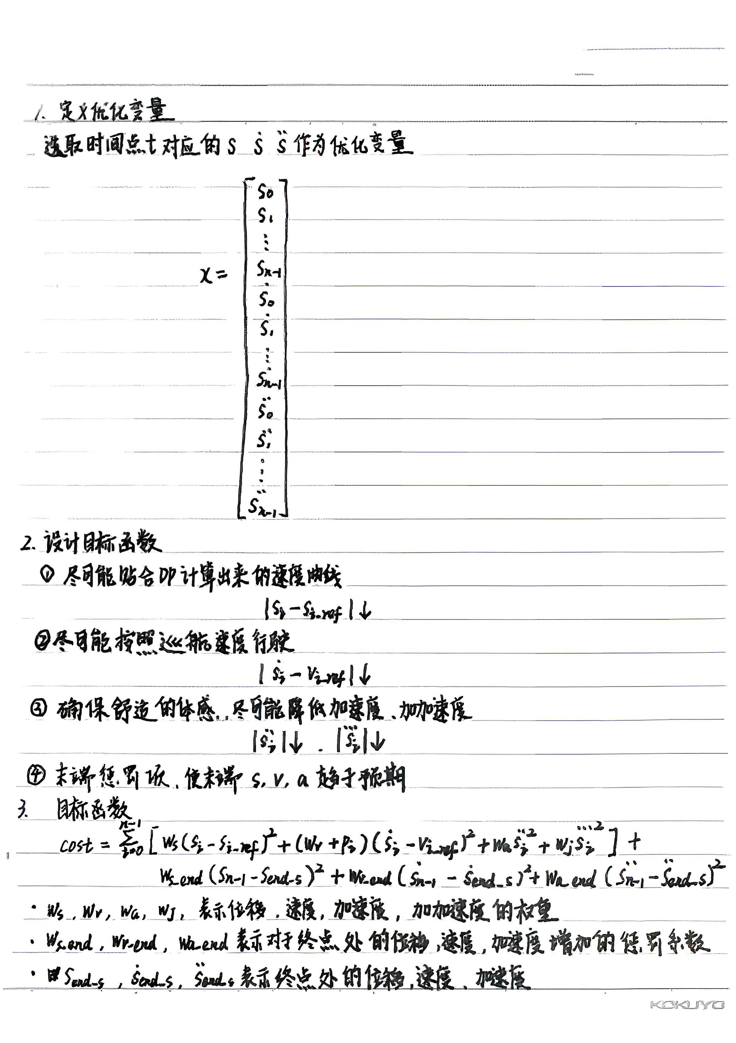
创建三维数组存储车辆的初始运动状态:位置,速度,加速度
const auto& vehicle_state = frame_->vehicle_state();
if (vehicle_state.gear() == canbus::Chassis::GEAR_REVERSE) {
  init_s[1] = std::max(-init_s[1], 0.0);
  init_s[2] = -init_s[2];
}
倒车状态处理
核心思想是将倒车映射为“正向运动” ,从而复用正向优化算法
double delta_t = 0.1;
double total_length = st_graph_data.path_length();
double total_time = st_graph_data.total_time_by_conf();
int num_of_knots = static_cast<int>(total_time / delta_t) + 1;
delta_t:时间步长固定为 0.1 秒 ,即每 0.1 秒取一个离散时间点
total_length:路径总长度从st_graph_data获取,表示本次规划路径的总长(米)
total_time:规划总时间由配置文件决定,表示本次速度规划覆盖的时间范围(秒)
num_of_knots:时间节点数根据总时间和步长计算, +1 确保包含起始时刻(t=0)
将连续的时间轴离散化为一系列等间隔的时刻,后续将在这些时刻上计算位置 s 的上下界约束
const double kEpsilon = 0.01;
  std::vector<std::pair<double, double>> s_bounds;
  for (int i = 0; i < num_of_knots; ++i) {
遍历时间点
 double curr_t = i * delta_t;
 double s_lower_bound = 0.0;
 double s_upper_bound = total_length;
 for (const STBoundary* boundary : st_graph_data.st_boundaries()) {
   double s_lower = 0.0;
   double s_upper = 0.0;
遍历ST图数据中的ST边界
GetUnblockSRange函数
if (!boundary->GetUnblockSRange(curr_t, &s_upper, &s_lower)) {
        continue;
      }
size_t left = 0;
  size_t right = 0;
  if (!GetIndexRange(lower_points_, curr_time, &left, &right)) {
    AERROR << "Fail to get index range.";
    return false;
  }
在lower_points_(下边界点序列)中查找时间区间 [left, right] ,使得 curr_time 落在这个区间内
if (curr_time > upper_points_[right].t()) {
  return true;
}
返回true, 表示整个s范围都未被阻挡
 const double r =
    (left == right
         ? 0.0
         : (curr_time - upper_points_[left].t()) /
               (upper_points_[right].t() - upper_points_[left].t()));
- 作用:计算当前时间curr_time在离散时间区间 [left, right] 中的相对位置
- 范围:0 ≤ r ≤ 1 , r=0 表示在左端点, r=1 表示在右端点
- 特殊情况:left == right 时 r=0.0(正好落在离散点上)
double upper_cross_s = upper_points_[left].s() + r * (upper_points_[right].s() - upper_points_[left].s());
double lower_cross_s = lower_points_[left].s() + r * (lower_points_[right].s() - lower_points_[left].s());
线性插值,得到障碍物在curr_time时刻占据的s范围[lower_cross_s, upper_cross_s]
if (boundary_type_ == BoundaryType::STOP ||
      boundary_type_ == BoundaryType::YIELD ||
      boundary_type_ == BoundaryType::FOLLOW) {
    *s_upper = lower_cross_s;
  } else if (boundary_type_ == BoundaryType::OVERTAKE) {
    *s_lower = std::fmax(*s_lower, upper_cross_s);
  }
- STOP/YIELD/FOLLOW : *s_upper = lower_cross_s
- 自车必须停在障碍物后方
- OVERTAKE : *s_lower = std::fmax(*s_lower, upper_cross_s)
- 自车必须超越障碍物前缘
s_bounds.emplace_back(s_lower_bound, s_upper_bound);
将当前时间点的s上下界约束(s_lower_bound, s_upper_bound)存入s_bounds向量
std::vector<double> x_ref(num_of_knots, total_length);
创建长度为num_of_knots的向量,所有元素初始化为total_length
std::vector<double> dx_ref(num_of_knots, reference_line_info_->GetCruiseSpeed());
创建速度参考向量,所有元素初始化为巡航速度
std::vector<double> dx_ref_weight(num_of_knots, config_.ref_v_weight());
创建速度权重向量,所有元素初始化为配置的权重值
std::vector<double> penalty_dx;
存储对速度偏差的惩罚值
std::vector<std::pair<double, double>> s_dot_bounds;
定义每个时间点允许的速度范围
const SpeedLimit& speed_limit = st_graph_data.speed_limit();
获取ST图中预计算的速度限制
for (int i = 0; i < num_of_knots; ++i) {
  double curr_t = i * delta_t;  // 当前时间点
遍历时间节点
SpeedPoint sp;
reference_speed_data.EvaluateByTime(curr_t, &sp);
const double path_s = sp.s();
x_ref[i] = path_s;
从speed_data中获取当前时间对应的s位置
PathPoint path_point = path_data.GetPathPointWithPathS(path_s);
penalty_dx.push_back(std::fabs(path_point.kappa()) *
                     config_.kappa_penalty_weight());
计算曲率惩罚penalty_dx
const double v_lower_bound = 0.0;
double v_upper_bound = FLAGS_planning_upper_speed_limit;
v_upper_bound =
    std::fmin(speed_limit.GetSpeedLimitByS(path_s), v_upper_bound);
dx_ref[i] = std::fmin(v_upper_bound, dx_ref[i]);
s_dot_bounds.emplace_back(v_lower_bound, std::fmax(v_upper_bound, 0.0));
速度边界计算与存储:
下界:0.0(不能倒车)
上界:取全局上限和路径点限制的最小值
参考速度:限制在允许范围内
存储:(0.0, 上界)存入s_dot_bounds
AdjustInitStatus函数
验证初始速度/加速度是否能在 jerk 约束下满足后续所有速度边界,如果不满足则将初始加速度调整为0
double v_min = init_s[1];  // 初始速度
double v_max = init_s[1];
double a_min = init_s[2];  // 初始加速度
double a_max = init_s[2];
for (size_t i = 1; i < s_dot_bound.size(); i++)
遍历所有时间点
// 保存上一时刻加速度
last_a_min = a_min;
last_a_max = a_max;
// 按最大/最小 jerk 推算新加速度
a_min = a_min + delta_t * FLAGS_longitudinal_jerk_upper_bound;
a_max = a_max + delta_t * FLAGS_longitudinal_jerk_lower_bound;
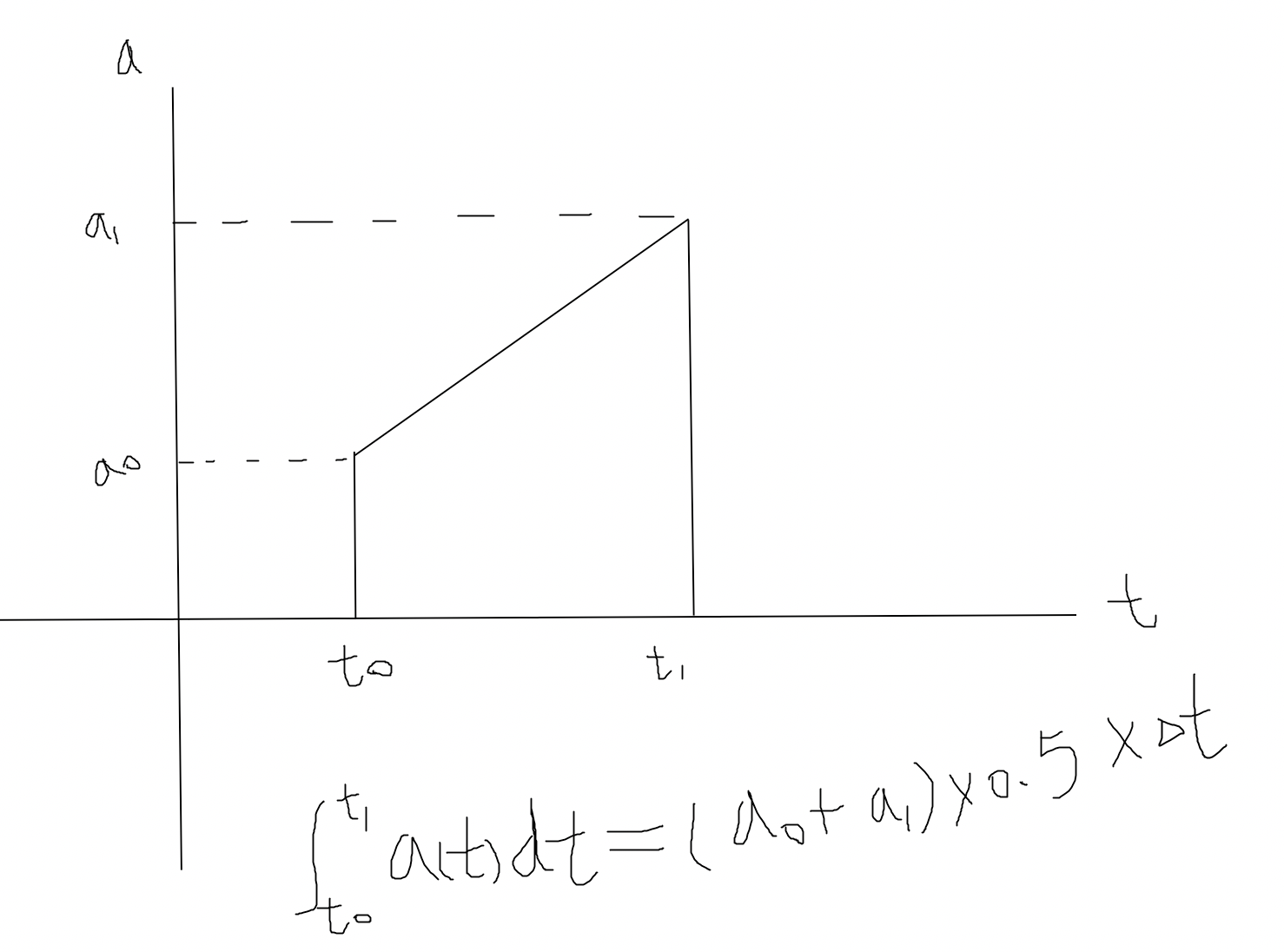
// 梯形积分法推算速度
v_min = v_min + 0.5 * delta_t * (a_min + last_a_min);
v_max = v_max + 0.5 * delta_t * (a_max + last_a_max);
if (v_min < s_dot_bound[i].first || v_max > s_dot_bound[i].second) {
  // 超出速度边界
  init_s[2] = 0;  // 将初始加速度设为 0
  return;
}
梯形积分法
表示速度的变化量
PiecewiseJerkSpeedProblem piecewise_jerk_problem(num_of_knots, delta_t, init_s);
创建优化问题对象
- num_of_knots:时间节点数量
- delta_t:时间步长(0.1 秒)
- init_s:初始状态(位置,速度,加速度}
piecewise_jerk_problem.set_weight_ddx(config_.acc_weight());    // 加速度权重
piecewise_jerk_problem.set_weight_dddx(config_.jerk_weight());  // jerk 权重
piecewise_jerk_problem.set_scale_factor({1.0, 10.0, 100.0});    // 缩放因子
设置优化权重
piecewise_jerk_problem.set_x_bounds(0.0, total_length);         // 位置:0~路径总长
piecewise_jerk_problem.set_ddx_bounds(veh_param.max_deceleration(), // 加速度
                                      veh_param.max_acceleration());
piecewise_jerk_problem.set_dddx_bound(FLAGS_longitudinal_jerk_lower_bound, // jerk
                                      FLAGS_longitudinal_jerk_upper_bound);
设置全局边界
piecewise_jerk_problem.set_x_bounds(std::move(s_bounds)); // 每个时间点的位置边界
设置详细位置边界
piecewise_jerk_problem.set_dx_ref(dx_ref_weight, dx_ref);       // 速度参考值
piecewise_jerk_problem.set_x_ref(config_.ref_s_weight(), std::move(x_ref)); // 位置参考值
设置参考轨迹
piecewise_jerk_problem.set_penalty_dx(penalty_dx);              // 速度惩罚(曲率)
piecewise_jerk_problem.set_dx_bounds(std::move(s_dot_bounds));  // 速度边界
设置惩罚项和速度边界
Optimize函数
piecewise_jerk_problem.Optimize()
FormulateProblem函数
CalculateKernel函数
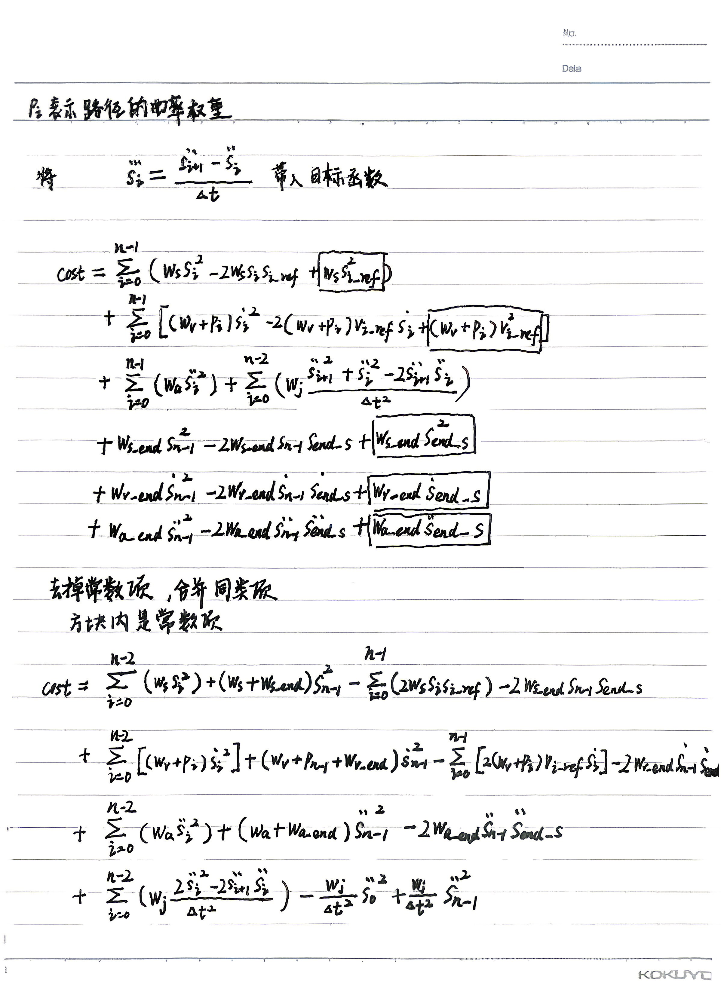
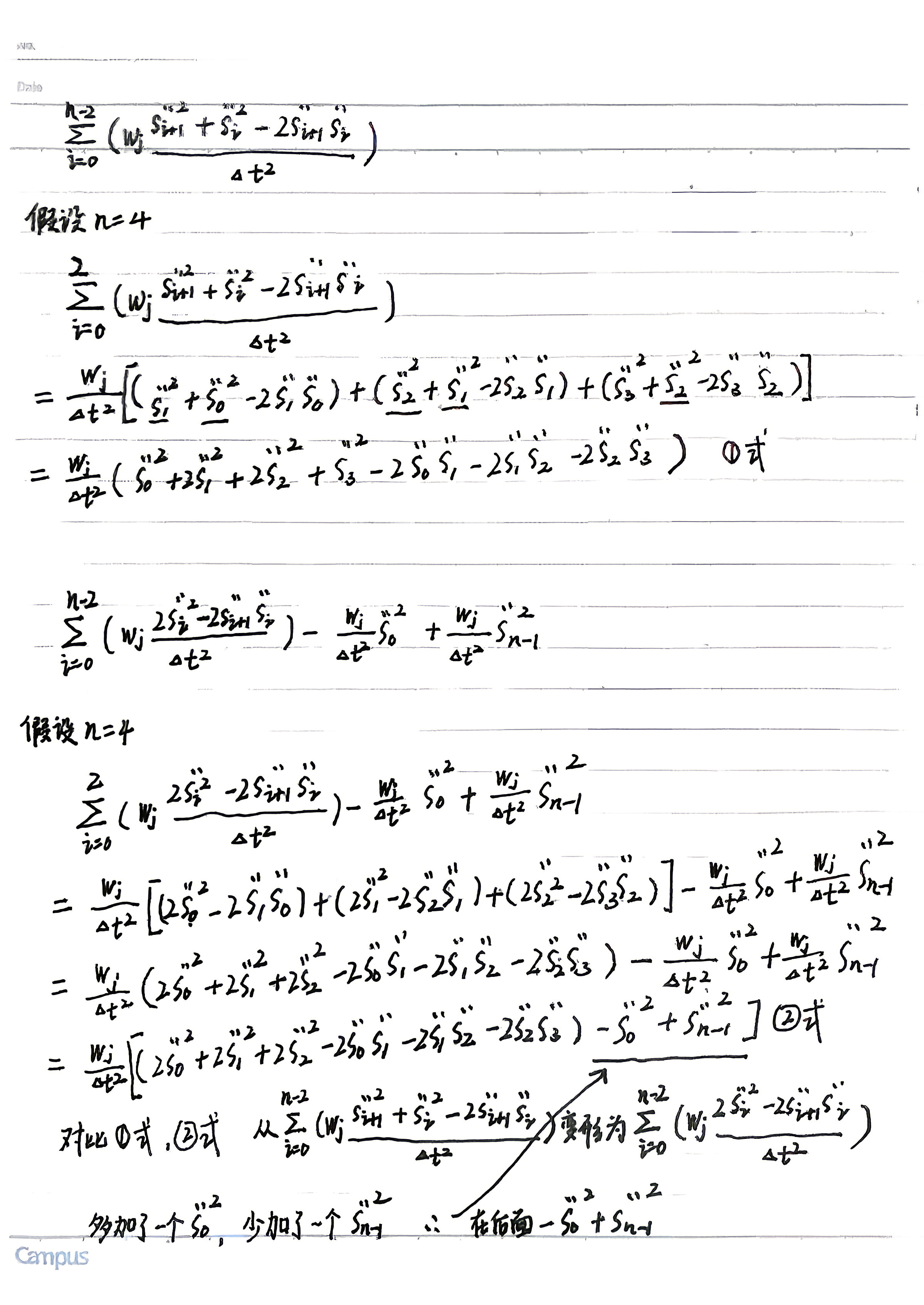
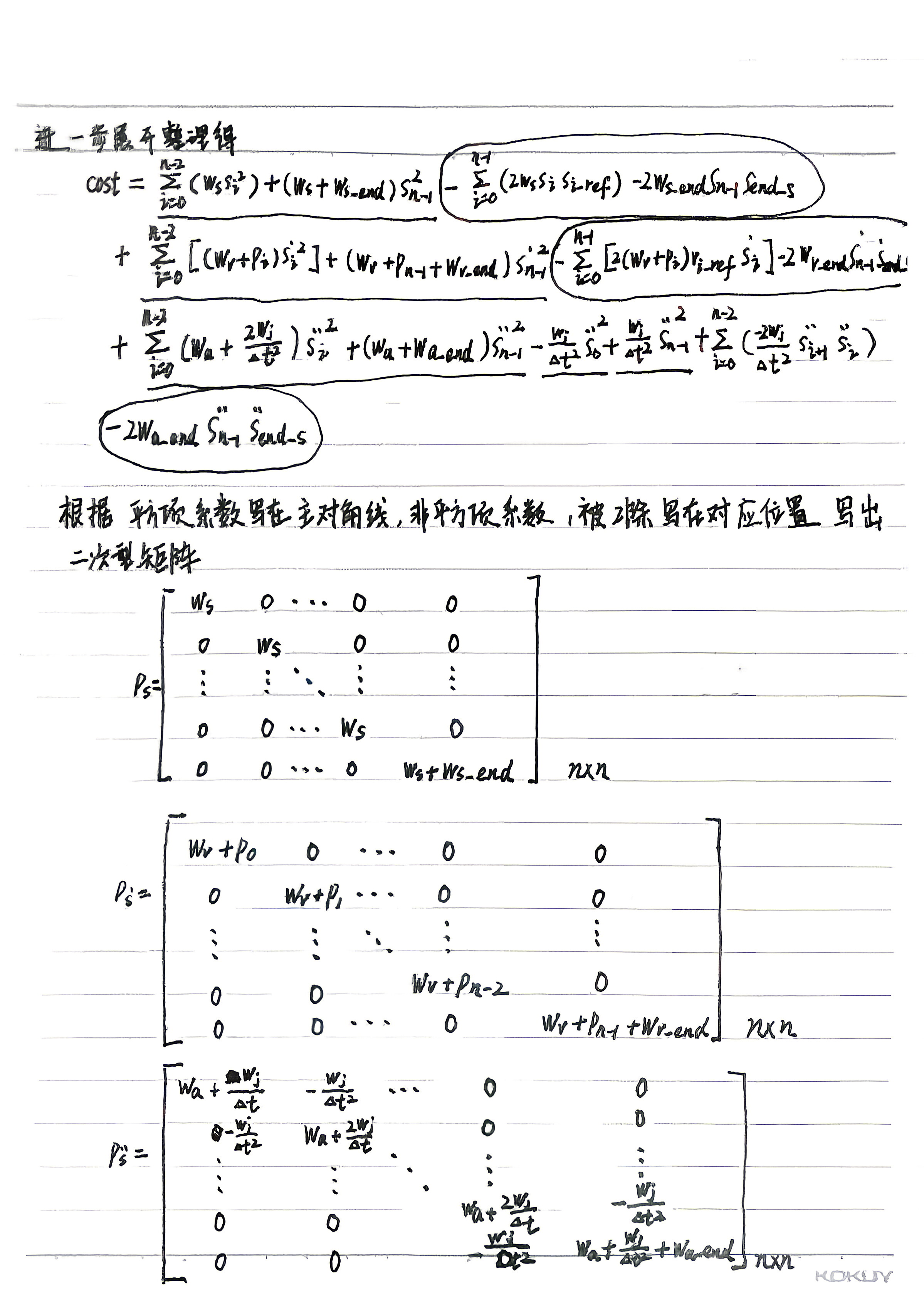
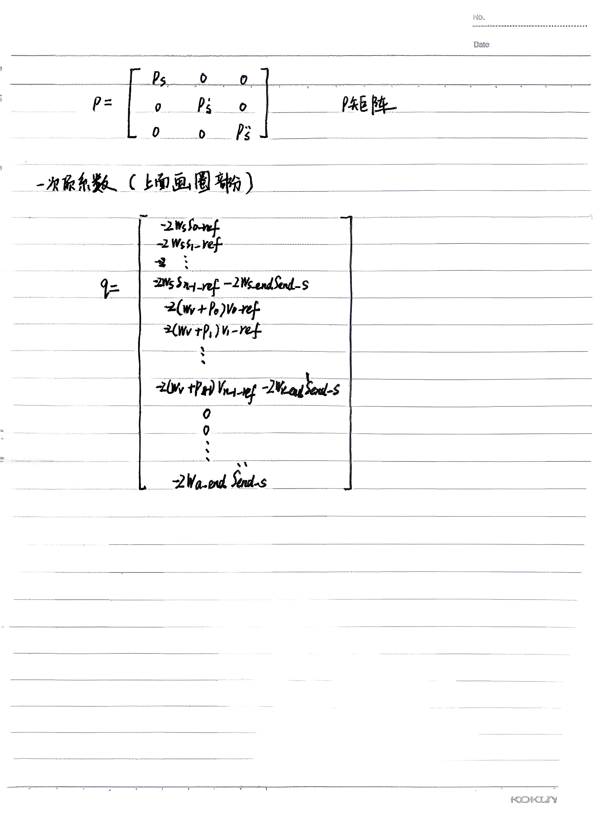
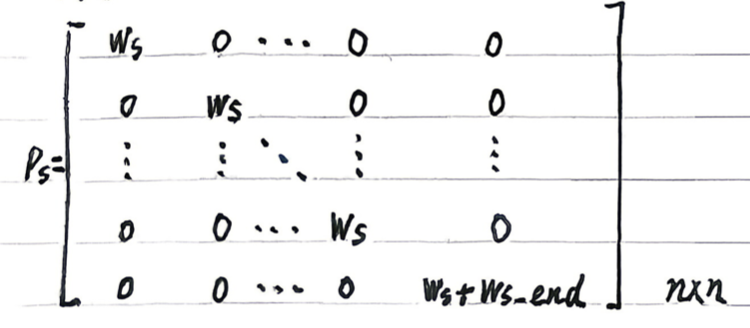
P矩阵
  for (int i = 0; i < n - 1; ++i) {
    columns[i].emplace_back(
        i, weight_x_ref_ / (scale_factor_[0] * scale_factor_[0]));
    ++value_index;
  }
[0, n - 2]主对角线系数
 columns[n - 1].emplace_back(n - 1, (weight_x_ref_ + weight_end_state_[0]) /
                                        (scale_factor_[0] * scale_factor_[0]));
[n - 1, n - 1]主对角线系数
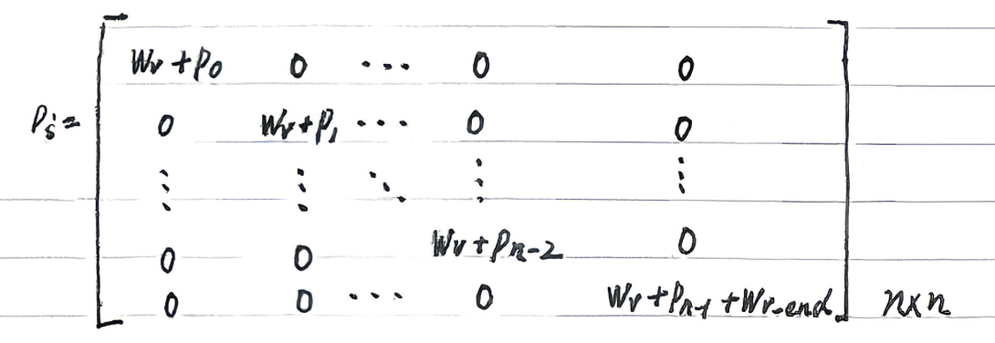
for (int i = 0; i < n - 1; ++i) {
    columns[n + i].emplace_back(n + i,
                                (weight_dx_ref_[i] + penalty_dx_[i]) /
                                    (scale_factor_[1] * scale_factor_[1]));
    ++value_index;
  }
[n, 2n-2]主对角线系数
columns[2 * n - 1].emplace_back(
      2 * n - 1,
      (weight_dx_ref_[n - 1] + penalty_dx_[n - 1] + weight_end_state_[1]) /
          (scale_factor_[1] * scale_factor_[1]));
[2n-1,2n-1]主对角线系数
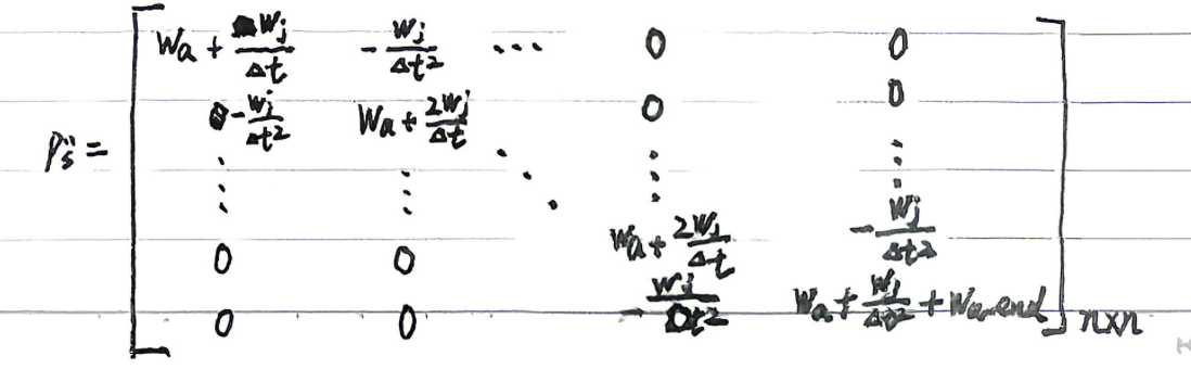
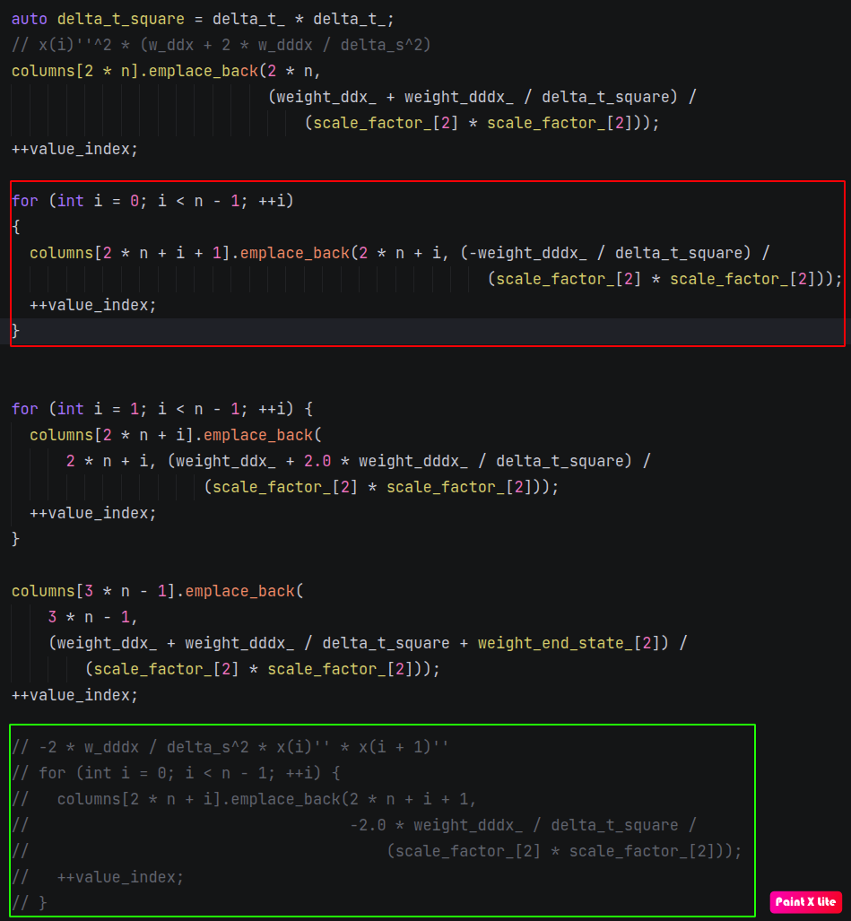
columns[2 * n].emplace_back(2 * n,
                              (weight_ddx_ + weight_dddx_ / delta_s_square) /
                                  (scale_factor_[2] * scale_factor_[2]));
[2n, 2n]
for (int i = 1; i < n - 1; ++i) {
    columns[2 * n + i].emplace_back(
        2 * n + i, (weight_ddx_ + 2.0 * weight_dddx_ / delta_s_square) /
                       (scale_factor_[2] * scale_factor_[2]));
    ++value_index;
  }
[2n + 1,3n-2]主对角线系数
columns[3 * n - 1].emplace_back(
      3 * n - 1,
      (weight_ddx_ + weight_dddx_ / delta_s_square + weight_end_state_[2]) /
          (scale_factor_[2] * scale_factor_[2]));
  ++value_index;
[3n - 1, 3n-1]
for (int i = 0; i < n - 1; ++i) {
  columns[2 * n + i].emplace_back(2 * n + i + 1,
                                  -2.0 * weight_dddx_ / delta_s_square /
                                      (scale_factor_[2] * scale_factor_[2]));
  ++value_index;
}
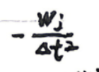
这块逻辑和planning模块(11)-路径规划优化算法(piecewise jerk path optimizer)相似同样是P矩阵交叉项系数计算错误,交叉项系数应该是
columns[col][row]是列行形式存储,

上面是P矩阵的存储过程
int ind_p = 0;
for (int i = 0; i < kNumParam; ++i) {
  P_indptr->push_back(ind_p);
  for (const auto& row_data_pair : columns[i]) {
    P_data->push_back(row_data_pair.second * 2.0);
    P_indices->push_back(row_data_pair.first);
    ++ind_p;
  }
}
P_indptr->push_back(ind_p);
上面是按照CSC矩阵存储规则进行存储
CSC(Compressed Sparse Column)矩阵
CalculateAffineConstraint函数
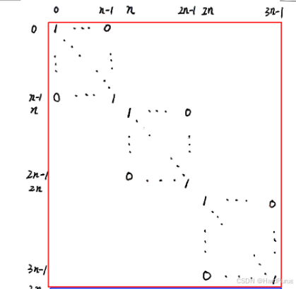
A矩阵
if (i < n) {
	 variables[i].emplace_back(constraint_index, 1.0);
	 lower_bounds->at(constraint_index) =
	     x_bounds_[i].first * scale_factor_[0];
	 upper_bounds->at(constraint_index) =
	     x_bounds_[i].second * scale_factor_[0];
	}
位置约束
x_bounds_[i].first ≤ x[i] ≤ x_bounds_[i].second
piecewise_jerk_problem.set_x_bounds(std::move(s_bounds));
else if (i < 2 * n) {
  variables[i].emplace_back(constraint_index, 1.0);
  lower_bounds->at(constraint_index) = dx_bounds_[i - n].first * scale_factor_[1];
  upper_bounds->at(constraint_index) = dx_bounds_[i - n].second * scale_factor_[1];
}
速度约束
dx_bounds_[i-n].first ≤ dx[i-n] ≤ dx_bounds_[i-n].second
piecewise_jerk_problem.set_dx_bounds(std::move(s_dot_bounds));
else {
  variables[i].emplace_back(constraint_index, 1.0);
  lower_bounds->at(constraint_index) = ddx_bounds_[i - 2 * n].first * scale_factor_[2];
  upper_bounds->at(constraint_index) = ddx_bounds_[i - 2 * n].second * scale_factor_[2];
}
加速度约束
ddx_bounds_[i-2n].first ≤ ddx[i-2n] ≤ ddx_bounds_[i-2n].second
piecewise_jerk_problem.set_ddx_bounds(veh_param.max_deceleration(),
                                        veh_param.max_acceleration());
系数
for (int i = 0; i + 1 < n; ++i) {
  variables[2 * n + i].emplace_back(constraint_index, -1.0);
  variables[2 * n + i + 1].emplace_back(constraint_index, 1.0);
  lower_bounds->at(constraint_index) =
      dddx_bound_.first * delta_s_ * scale_factor_[2];
  upper_bounds->at(constraint_index) =
      dddx_bound_.second * delta_s_ * scale_factor_[2];
  ++constraint_index;
}
代码中delta_s_的应该是时间delta_t_由于速度二次规划和路径二次规划使用了同一个基类,所以在二次规划中也沿用了delta_s_=1.0,来表示delta_t
加加速度约束
Jerk \approx\frac{\ddot{x_{i+1}}-\ddot{x_{i}}}{\Delta t}
// Jerk ≈ 相邻加速度的差分
jerk[i] = (- ddx[i]+ ddx[i+1]) / delta_t

// 约束:
jerk_min ≤ (- ddx[i]+ ddx[i+1]) / delta_t ≤ jerk_max

// 两边同乘 delta_t:
jerk_min * delta_t ≤ - ddx[i]+ ddx[i+1] ≤ jerk_max * delta_t
piecewise_jerk_problem.set_dddx_bound(FLAGS_longitudinal_jerk_lower_bound,
                                        FLAGS_longitudinal_jerk_upper_bound);
系数
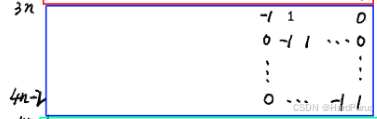
for (int i = 0; i + 1 < n; ++i) {
  variables[n + i].emplace_back(constraint_index, -1.0 * scale_factor_[2]);
  variables[n + i + 1].emplace_back(constraint_index, 1.0 * scale_factor_[2]);
  variables[2 * n + i].emplace_back(constraint_index,
                                    -0.5 * delta_s_ * scale_factor_[1]);
  variables[2 * n + i + 1].emplace_back(constraint_index,
                                        -0.5 * delta_s_ * scale_factor_[1]);
  lower_bounds->at(constraint_index) = 0.0;
  upper_bounds->at(constraint_index) = 0.0;
  ++constraint_index;
}
速度连续性约束
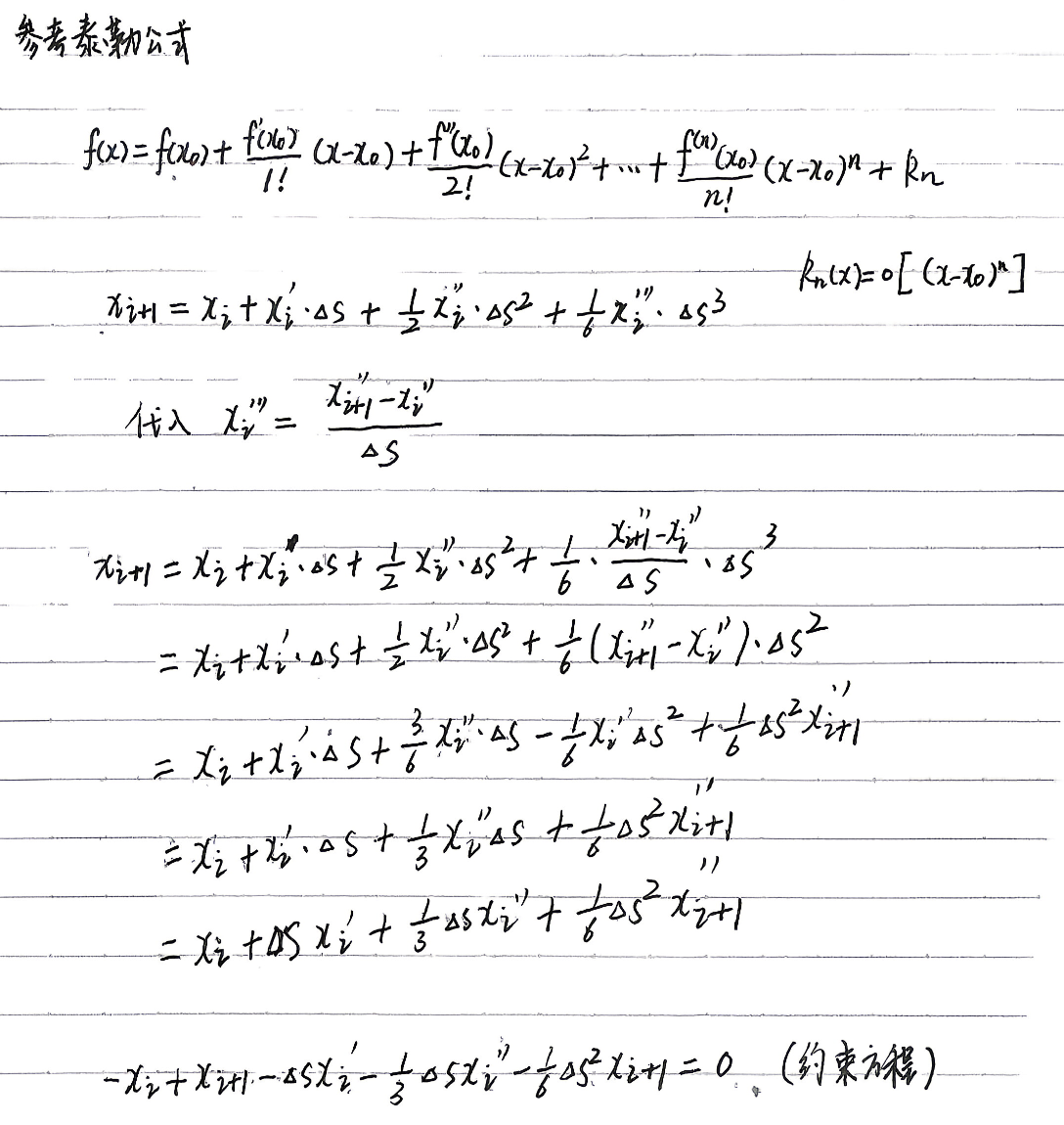
\dot{x_{i+1}}=\dot{x_{i}}+\int_{t_{i}}^{t_{i+1}}\ddot{x(t)}dt\approx \dot{x_{i}}+\frac{\ddot{x_{i}}+\ddot{x_{i+1}}}{2}\Delta t
\int_{t_{i}}^{t_{i+1}}\ddot{x(t)}dt\approx \frac{\ddot{x_{i}}+\ddot{x_{i+1}}}{2}\Delta t(梯形积分法,使用梯形面积近似积分结果)
整理成约束方程的形式:
-\dot{x_{i}}+\dot{x_{i+1}}-\frac{1}{2}\Delta{t}(\ddot{x_{i}}+\ddot{x_{i+1}})=0
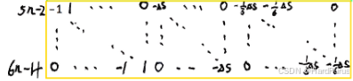
系数
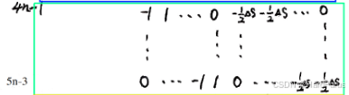
图片中\Delta s变为\Delta t
auto delta_s_sq_ = delta_s_ * delta_s_;
  for (int i = 0; i + 1 < n; ++i) {
    variables[i].emplace_back(constraint_index,
                              -1.0 * scale_factor_[1] * scale_factor_[2]);
    variables[i + 1].emplace_back(constraint_index,
                                  1.0 * scale_factor_[1] * scale_factor_[2]);
    variables[n + i].emplace_back(
        constraint_index, -delta_s_ * scale_factor_[0] * scale_factor_[2]);
    variables[2 * n + i].emplace_back(
        constraint_index,
        -delta_s_sq_ / 3.0 * scale_factor_[0] * scale_factor_[1]);
    variables[2 * n + i + 1].emplace_back(
        constraint_index,
        -delta_s_sq_ / 6.0 * scale_factor_[0] * scale_factor_[1]);

    lower_bounds->at(constraint_index) = 0.0;
    upper_bounds->at(constraint_index) = 0.0;
    ++constraint_index;
  }
位置、加速度连续性约束
系数
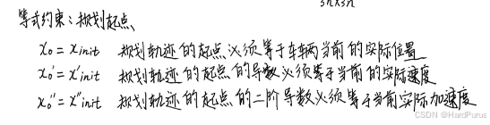
  variables[0].emplace_back(constraint_index, 1.0);
  lower_bounds->at(constraint_index) = x_init_[0] * scale_factor_[0];
  upper_bounds->at(constraint_index) = x_init_[0] * scale_factor_[0];
  ++constraint_index;

  variables[n].emplace_back(constraint_index, 1.0);
  lower_bounds->at(constraint_index) = x_init_[1] * scale_factor_[1];
  upper_bounds->at(constraint_index) = x_init_[1] * scale_factor_[1];
  ++constraint_index;

  variables[2 * n].emplace_back(constraint_index, 1.0);
  lower_bounds->at(constraint_index) = x_init_[2] * scale_factor_[2];
  upper_bounds->at(constraint_index) = x_init_[2] * scale_factor_[2];
  ++constraint_index;
  int ind_p = 0;
  for (int i = 0; i < num_of_variables; ++i) {
    A_indptr->push_back(ind_p);
    for (const auto& variable_nz : variables[i]) {
      // coefficient
      A_data->push_back(variable_nz.second);

      // constraint index
      A_indices->push_back(variable_nz.first);
      ++ind_p;
    }
  }
  // We indeed need this line because of
  // https://github.com/oxfordcontrol/osqp/blob/master/src/cs.c#L255
  A_indptr->push_back(ind_p);
csc存储
CalculateOffset函数
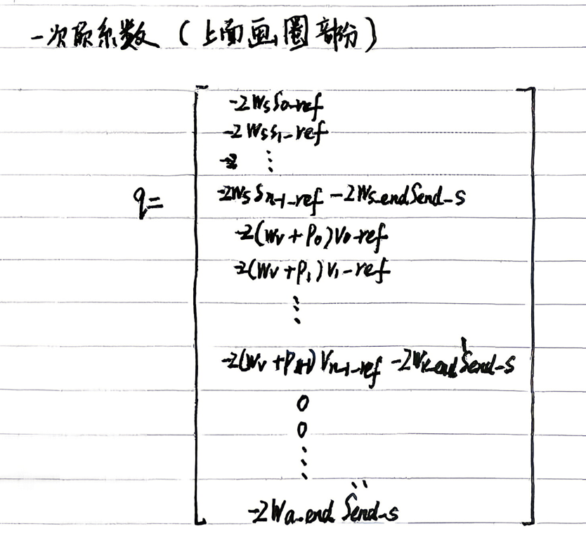
Q矩阵
void PiecewiseJerkSpeedProblem::CalculateOffset(std::vector<c_float>* q) {
  CHECK_NOTNULL(q);
  const int n = static_cast<int>(num_of_knots_);
  const int kNumParam = 3 * n;
  q->resize(kNumParam);
  for (int i = 0; i < n; ++i) {
    if (has_x_ref_) {
      q->at(i) += -2.0 * weight_x_ref_ * x_ref_[i] / scale_factor_[0];
    }
    if (has_dx_ref_) {
      q->at(n + i) += -2.0 * weight_dx_ref_[i] * dx_ref_[i] / scale_factor_[1];
    }
  }

  if (has_end_state_ref_) {
    q->at(n - 1) +=
        -2.0 * weight_end_state_[0] * end_state_ref_[0] / scale_factor_[0];
    q->at(2 * n - 1) +=
        -2.0 * weight_end_state_[1] * end_state_ref_[1] / scale_factor_[1];
    q->at(3 * n - 1) +=
        -2.0 * weight_end_state_[2] * end_state_ref_[2] / scale_factor_[2];
  }
}
这里Q矩阵速度项忽略了p_{i}曲率惩罚系数
size_t kernel_dim = 3 * num_of_knots_;
优化变量的总数
size_t num_affine_constraint = lower_bounds.size();
CalculateAffineConstraint中约束总数
data->n = kernel_dim;
设置OSQP优化变量数量
data->m = num_affine_constraint;
设置OSQP约束数量
data->P = csc_matrix(kernel_dim, kernel_dim, P_data.size(),
                     CopyData(P_data), CopyData(P_indices), CopyData(P_indptr));
构建目标函数矩阵P
- csc_matrix :创建 压缩稀疏列 (CSC) 格式的矩阵
- 参数 :
- kernel_dim, kernel_dim :P 是 n × n 的方阵(3n × 3n)
- P_data.size() :非零元素个数
- CopyData(P_data) :非零元素值数组
- CopyData(P_indices) :行索引数组
- CopyData(P_indptr) :列指针数组
data->q = CopyData(q);
设置目标函数线性项
data->A = csc_matrix(num_affine_constraint, kernel_dim, A_data.size(),
                     CopyData(A_data), CopyData(A_indices), CopyData(A_indptr));
构建约束矩阵 A
data->l = CopyData(lower_bounds);
设置约束下界
data->u = CopyData(upper_bounds);
设置约束上界
return CheckLowUpperBound(lower_bounds, upper_bounds);
验证约束合法性
OSQPSettings* settings = SolverDefaultSettings();
获取OSQP求解器的默认配置
settings->max_iter = max_iter;
设置最大迭代次数,默认是4000
OSQPWorkspace* osqp_work = nullptr;
声明工作空间指针
osqp_work = osqp_setup(data, settings);
初始化求解器
参数 :
- data :问题定义(P, q, A, l, u 矩阵)
- settings :求解器配置
osqp_solve(osqp_work);
执行优化求解
运行ADMM(交替方向乘子法)求解二次规划问题
auto status = osqp_work->info->status_val;
获取求解状态
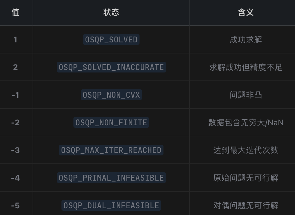
if (status < 0 || (status != 1 && status != 2)) {
  AERROR << "failed optimization status:\t" << osqp_work->info->status;
  osqp_cleanup(osqp_work);
  FreeData(data);
  c_free(settings);
  return false;
}
检查求解状态
} else if (osqp_work->solution == nullptr) {
  AERROR << "The solution from OSQP is nullptr";
  osqp_cleanup(osqp_work);
  FreeData(data);
  c_free(settings);
  return false;
}
即使状态码正常,解指针也可能为空
// extract primal results
x_.resize(num_of_knots_);
dx_.resize(num_of_knots_);
ddx_.resize(num_of_knots_);
- x_ :位置轨迹(s)
- dx_ :速度轨迹(v)
- ddx_ :加速度轨迹(a)
for (size_t i = 0; i < num_of_knots_; ++i) {
  x_.at(i) = osqp_work->solution->x[i] / scale_factor_[0];
  dx_.at(i) = osqp_work->solution->x[i + num_of_knots_] / scale_factor_[1];
  ddx_.at(i) =
      osqp_work->solution->x[i + 2 * num_of_knots_] / scale_factor_[2];
}
提取并反缩放结果
// Cleanup
osqp_cleanup(osqp_work);
FreeData(data);
c_free(settings);
return true;
- osqp_cleanup :释放求解器工作空间(最重要)
- FreeData :释放问题数据矩阵(P, A 等)
- c_free :释放配置参数
到这Optimize函数就介绍完了
const std::vector<double>& s = piecewise_jerk_problem.opt_x();
const std::vector<double>& ds = piecewise_jerk_problem.opt_dx();
const std::vector<double>& dds = piecewise_jerk_problem.opt_ddx();
获取优化结果
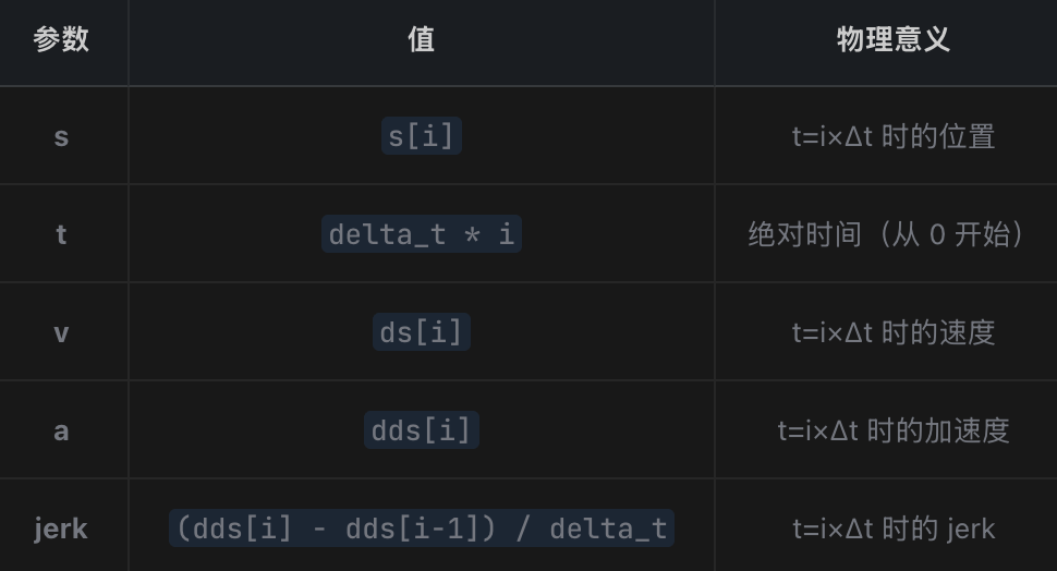
- s :优化后的 位置轨迹 (s[i] 表示 t=i×Δt 时的位置)
- ds :优化后的 速度轨迹 (ds[i] 表示 t=i×Δt 时的速度)
- dds :优化后的 加速度轨迹 (dds[i] 表示 t=i×Δt 时的加速度)
for (int i = 1; i < num_of_knots; ++i) {
  // Avoid the very last points when already stopped
  if (ds[i] <= 0.0) {
    break;
  }
  speed_data->AppendSpeedPoint(s[i], delta_t * i, ds[i], dds[i],
                               (dds[i] - dds[i - 1]) / delta_t);
}
遍历添加速度点
SpeedProfileGenerator::FillEnoughSpeedPoints(speed_data);
填充足够的速度点
到这PIECEWISE_JERK_SPEED task就介绍完了
然后CombinePathAndSpeedProfile函数会被调用
modules/planning/scenarios/lane_follow/lane_follow_stage.cc
CombinePathAndSpeedProfile函数
reference_line_info.CombinePathAndSpeedProfile(
            planning_start_point.relative_time(),
            planning_start_point.path_point().s(), &trajectory)
speed_data_.EvaluateByTime(cur_rel_time, &speed_point)
速度点插值
common::PathPoint path_point =
    path_data_.GetPathPointWithPathS(speed_point.s());
path_point.set_s(path_point.s() + start_s);

common::TrajectoryPoint trajectory_point;
trajectory_point.mutable_path_point()->CopyFrom(path_point);
trajectory_point.set_v(speed_point.v());
trajectory_point.set_a(speed_point.a());
trajectory_point.set_relative_time(speed_point.t() + relative_time);
ptr_discretized_trajectory->AppendTrajectoryPoint(trajectory_point);
构建轨迹点
 if (path_data_.is_reverse_path()) {
   std::for_each(ptr_discretized_trajectory->begin(),
                 ptr_discretized_trajectory->end(),
                 [](common::TrajectoryPoint& trajectory_point) {
                   trajectory_point.set_v(-trajectory_point.v());
                   trajectory_point.set_a(-trajectory_point.a());
                   trajectory_point.mutable_path_point()->set_s(
                       -trajectory_point.path_point().s());
                 });
   AINFO << "reversed path";
   ptr_discretized_trajectory->SetIsReversed(true);
 }
倒车处理,度、加速度和路径长度都取反
last_publishable_trajectory_.reset(new PublishableTrajectory(
        current_time_stamp, best_ref_info->trajectory()));
last_publishable_trajectory_->PopulateTrajectoryProtobuf(ptr_trajectory_pb);

void PublishableTrajectory::PopulateTrajectoryProtobuf(
    ADCTrajectory* trajectory_pb) const {
  CHECK_NOTNULL(trajectory_pb);
  trajectory_pb->mutable_header()->set_timestamp_sec(header_time_);
  trajectory_pb->mutable_trajectory_point()->CopyFrom({begin(), end()});
在PopulateTrajectoryProtobuf函数中将轨迹点赋值给了ptr_trajectory_pb
然后通过出参
  auto status = planner_->Plan(stitching_trajectory.back(), frame_.get(),
                               ptr_trajectory_pb);
status = Plan(start_timestamp, stitching_trajectory, ptr_trajectory_pb);
planning_base_->RunOnce(local_view_, &adc_trajectory_pb);
返回adc_trajectory_pb
planning_writer_->Write(adc_trajectory_pb);
然后将轨迹发出,给control模块使用