
本篇将介绍路径规划piecewise jerk path optimizer(分段加加速度路径优化算法)
上一篇planning模块-基于静态障碍物进一步缩放路径边界 已经介绍完了DecidePathBounds函数.
本篇将介绍OptimizePath函数
OptimizePath函数
bool LaneFollowPath::OptimizePath(
    const std::vector<PathBoundary>& path_boundaries,
    std::vector<PathData>* candidate_path_data)
path_boundaries:是通过DecidePathBounds函数获取到的基于静态障碍物进一步缩放的路径边界
const auto& config = config_.path_optimizer_config();
读取的是modules/planning/tasks/lane_follow_path/conf/default_conf.pb.txt路径下的配置
is_extend_lane_bounds_to_include_adc: true
extend_buffer: 0.2
path_optimizer_config {
  l_weight: 1.0
  dl_weight: 20.0
  ddl_weight: 1000.0
  dddl_weight: 50000.0
  lateral_derivative_bound_default: 2.0
  path_reference_l_weight:100
}
| 配置项 | 作用对象 | 数学/物理含义 | 直觉解释 | 调大后的效果 | 调小后的效果 |
|---|---|---|---|---|---|
is_extend_lane_bounds_to_include_adc |
车道边界 | 扩展可行解空间 | 保证自车一定在可行域内 | 更稳,不易无解 | 可能一开始就无解 |
extend_buffer |
车道边界 | 边界安全裕量(m) | 给车道留点余量 | 更保守,离边界远 | 易贴边、受噪声影响 |
l_weight |
l(s) |
横向偏移惩罚 | 别离中线太远 | 更靠近中心线 | 更自由横向偏移 |
dl_weight |
dl/ds |
横向坡度 | 抑制突然偏移 | 方向更平缓 | 容易斜切 |
ddl_weight |
d²l/ds² |
曲率 / 横向加速度 | 抑制急转弯 | 更舒适 | 转向更激进 |
dddl_weight |
d³l/ds³ |
曲率变化率 / jerk | 防抖、防鬼畜 | 极度平顺 | 方向盘抖动 |
lateral_derivative_bound_default |
dl/ds |
硬约束上限 | 限制最大横向倾斜 | 路径更保守 | 可横穿车道 |
path_reference_l_weight |
l - l_ref |
贴参考线惩罚 | 跟着参考线走 | 路径死板 | 路径更灵活 |
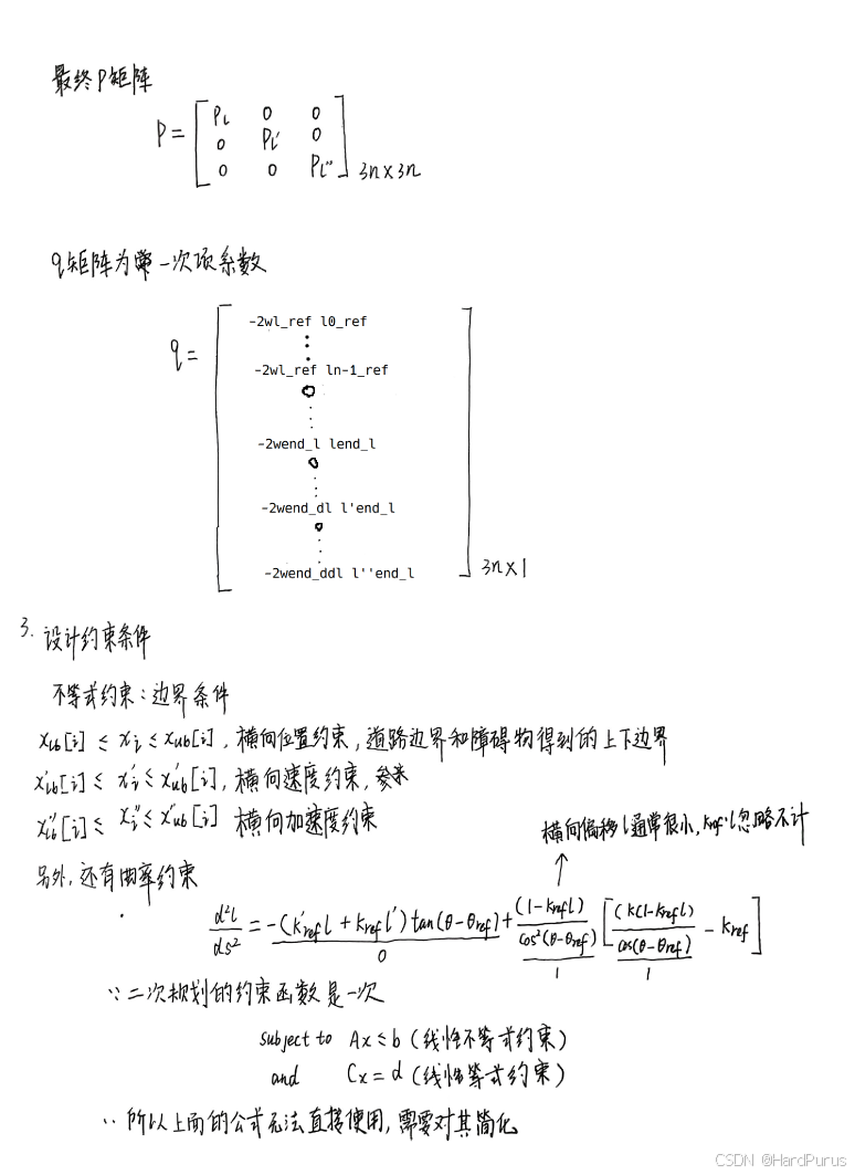
CalculateAccBound函数
const double lat_acc_bound =
    std::tan(veh_param.max_steer_angle() / veh_param.steer_ratio()) /
    veh_param.wheel_base();
veh_param.max_steer_angle():方向盘最大转角
veh_param.steer_ratio():转向传动比
veh_param.wheel_base():轴距
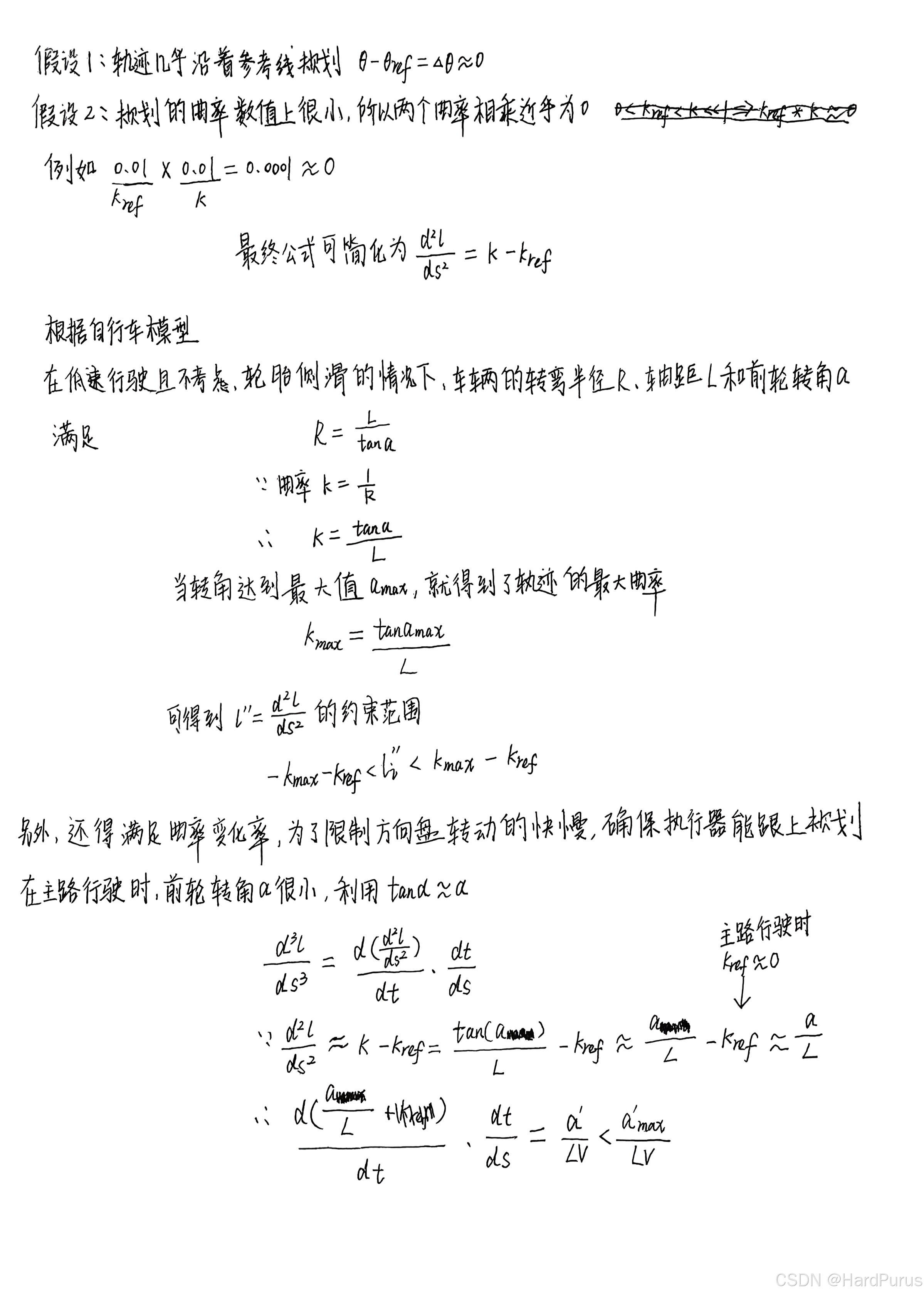
基于自行车模型,车辆的曲率 k 与前轮转角 \delta 的关系为 k = \frac{\tan(\delta)}{L},其中 L 是轴距
lat_acc_bound:实际上是车辆物理结构允许的最大曲率(单位:1/m),它限制了车轮能掰多大
for (size_t i = 0; i < path_boundary_size; ++i) {
    double s = static_cast<double>(i) * path_boundary.delta_s() + path_boundary.start_s();
    double kappa = reference_line.GetNearestReferencePoint(s).kappa();
    ...
}
s: 当前点在参考线上的累积距离
kappa (\kappa_{ref}): 获取参考线在 s 位置处的曲率
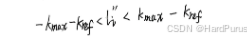
ddl_bounds->emplace_back(-lat_acc_bound - kappa, lat_acc_bound - kappa);
下面这个公式来自论文Optimal Trajectory Generation for Dynamic Street Scenarios in a Frene´t Frame感兴趣的可以看一下这篇论文.
下面是计算l''约束的过程,再解释一下k_{ref}l,简化为主干路行驶时,参考线的曲率很小,接近车道中心线,自车的横向偏移也很小基本是沿着参考线行驶,所以k_{ref}l\approx0
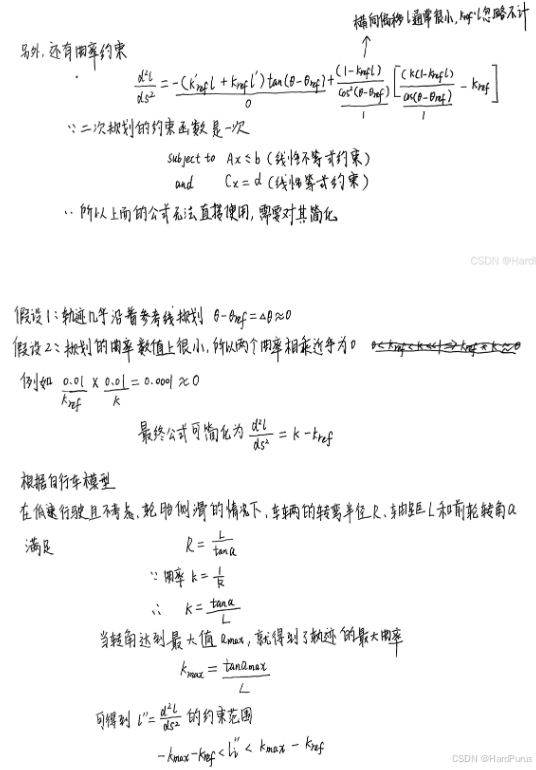
所以ddl_bounds它确定了路径优化时横向偏移量 l 对 s 的二阶导数的范围
到这CalculateAccBound函数就介绍完了
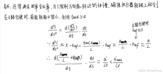
EstimateJerkBoundary函数
double PathOptimizerUtil::EstimateJerkBoundary(const double vehicle_speed) {
  const auto& veh_param =
      common::VehicleConfigHelper::GetConfig().vehicle_param();
  const double axis_distance = veh_param.wheel_base();
  const double max_yaw_rate =
      veh_param.max_steer_angle_rate() / veh_param.steer_ratio();
  return max_yaw_rate / axis_distance / vehicle_speed;
}
EstimateJerkBoundary函数主要是确定路径优化时横向偏移量 l 对 s 的三阶导数的约束边界
veh_param.max_steer_angle_rate():最大方向盘转向速率,单位弧度每秒
veh_param.steer_ratio():转向传动比
max_yaw_rate:前轮转角的最大转向速率,就是\alpha _{max}',注意这里\alpha是前轮转角
axis_distance:轴距
max_yaw_rate / axis_distance / vehicle_speed:\frac{\alpha _{max}'}{Lv}
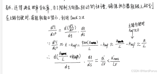
到这EstimateJerkBoundary函数就介绍完了
UpdatePathRefWithBound函数
当路被障碍物挤窄了,系统会临时产生一个新的“局部参考中心”
path_boundary:当前参考线长度对应的路径边界采样点信息
config.path_reference_l_weight():贴着参考线行驶的权重,默认为100
当左边界或右边界是由“障碍物”定义时,才考虑更新,简单说就是有车辆占了车辆左侧或右侧的可行驶空间,并且原始的理想参考中心towing_l已经不在当前车辆的路径边界范围内了,此时会更新新的参考中心,并更新权重
ref_l->at(i) =
          (path_boundary[i].l_lower.l + path_boundary[i].l_upper.l) / 2.0;
      weight_ref_l->at(i) = weight;
OptimizePath函数
init_state:规划起点的(s, s', s'',l, l',l'')
end_state:规划终点的(l, l', l''),都设为0,期待平稳回到参考中心
l_ref/l_ref_weight:通过函数UpdatePathRefWithBound计算出的参考中心,及其权重
path_boundary:路径边界采样点的信息
ddl_bounds:通过CalculateAccBound函数获取到的每一采样点允许的最大l''
dddl_bound:通过EstimateJerkBoundary函数获取到的允许的最大l'''
const auto& lat_boundaries = path_boundary.boundary();
const size_t kNumKnots = lat_boundaries.size();
double delta_s = path_boundary.delta_s();
  PiecewiseJerkPathProblem piecewise_jerk_problem(kNumKnots, delta_s,
                                                  init_state.second);
kNumKnots:路径边界采样点个数
delta_s:采样距离
init_state.second:规划起点的(l, l', l'')
因为FLAGS_enable_adc_vertex_constraint/FLAGS_enable_corner_constraint配置默认是false,所以
const auto& extra_bound = path_boundary.extra_path_bound();
const auto& adc_vertex_constraints = path_boundary.adc_vertex_bound();
adc_vertex_constraints/ extra_bound size是0
std::array<double, 3U> end_state_weight = {config.weight_end_state_l(),
                                             config.weight_end_state_dl(),
                                             config.weight_end_state_ddl()};
  piecewise_jerk_problem.set_end_state_ref(end_state_weight, end_state);
设置目标状态(l, l', l'')及其惩罚权重到piecewise_jerk_problem求解器
piecewise_jerk_problem.set_x_ref(std::move(l_ref_weight), l_ref);
  piecewise_jerk_problem.set_towing_x_ref(config.l_weight(), towing_l_ref);
set_x_ref:追踪由障碍物挤压后生成的“局部参考中心”.这保证了避障时的安全性.
set_towing_x_ref:追踪“原始全局参考中心”.
  piecewise_jerk_problem.set_weight_x(config.l_weight());
  piecewise_jerk_problem.set_weight_dx(config.dl_weight());
  piecewise_jerk_problem.set_weight_ddx(config.ddl_weight());
  piecewise_jerk_problem.set_weight_dddx(config.dddl_weight());
上述配置来自modules/planning/tasks/lane_follow_path/conf/default_conf.pb.txt
config.l_weight():偏离参考线的权重
config.dl_weight():侧向速度(斜率)的代价
config.ddl_weight():侧向加速度(曲率)的代价
config.dddl_weight():侧向加加速度(Jerk)的代价
piecewise_jerk_problem.set_scale_factor({1.0, 10.0, 100.0});
scale_factor:由于 l、l'、l'' 的数值量级不同(例如 l 可能是几米,而 l'' 可能只有 0.01)通过缩放因子将它们转化到同一量级,可以提高 QP 求解器的数值稳定性
  piecewise_jerk_problem.set_x_bounds(lat_boundaries);
  piecewise_jerk_problem.set_dx_bounds(
      -config.lateral_derivative_bound_default(),
      config.lateral_derivative_bound_default());
  piecewise_jerk_problem.set_ddx_bounds(ddl_bounds);

  piecewise_jerk_problem.set_dddx_bound(dddl_bound);
set_dx_bounds:对l的约束区域
set_ddx_bounds:对l''的约束区域
set_dddx_bound:对l'''的约束区域
Optimize函数
bool PiecewiseJerkProblem::Optimize(const int max_iter)
max_iter:最大迭代次数,默认是4000
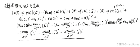
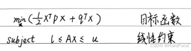
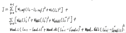
piecewise jerk path optimizer算法二次规划问题的构造如下:
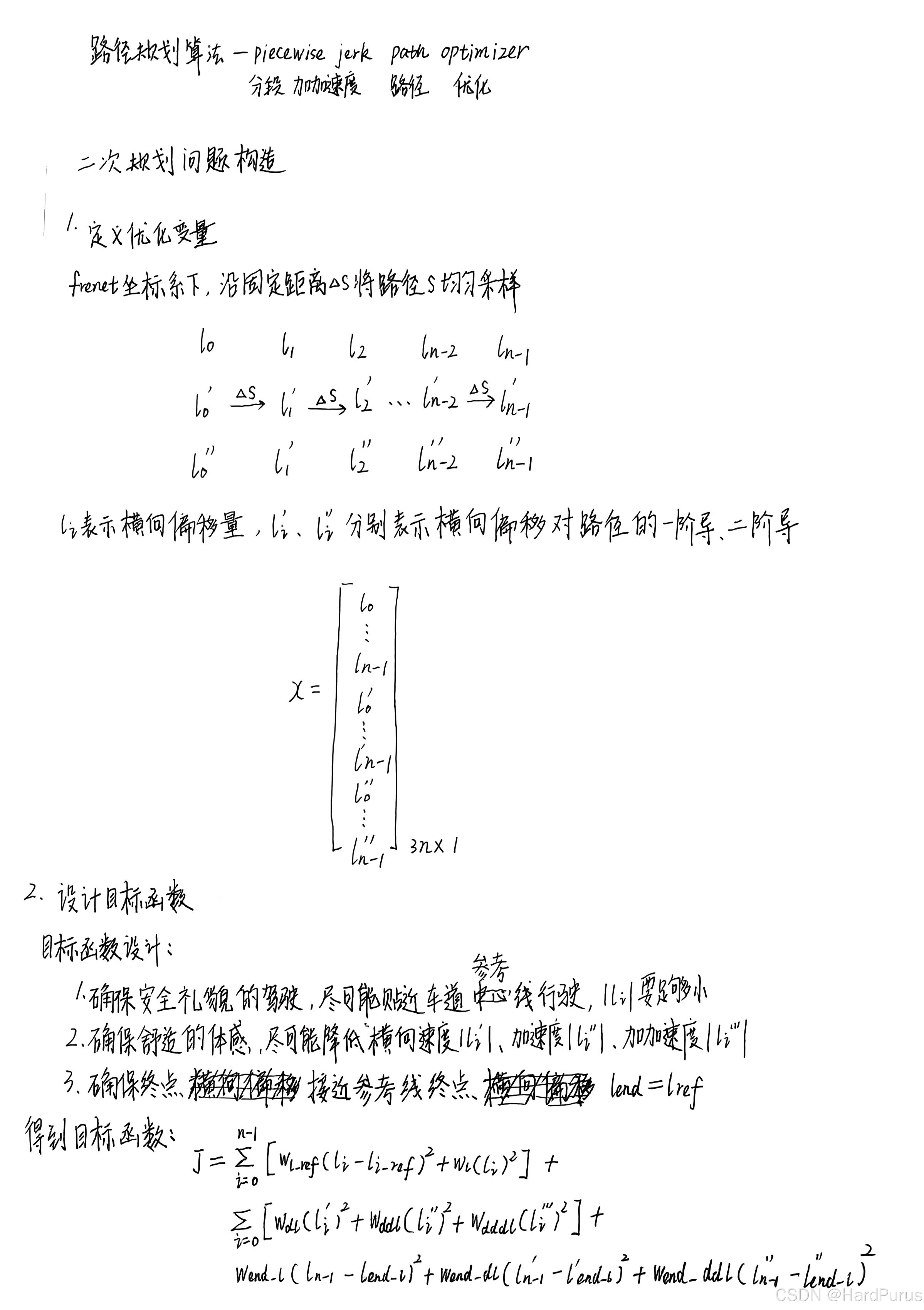
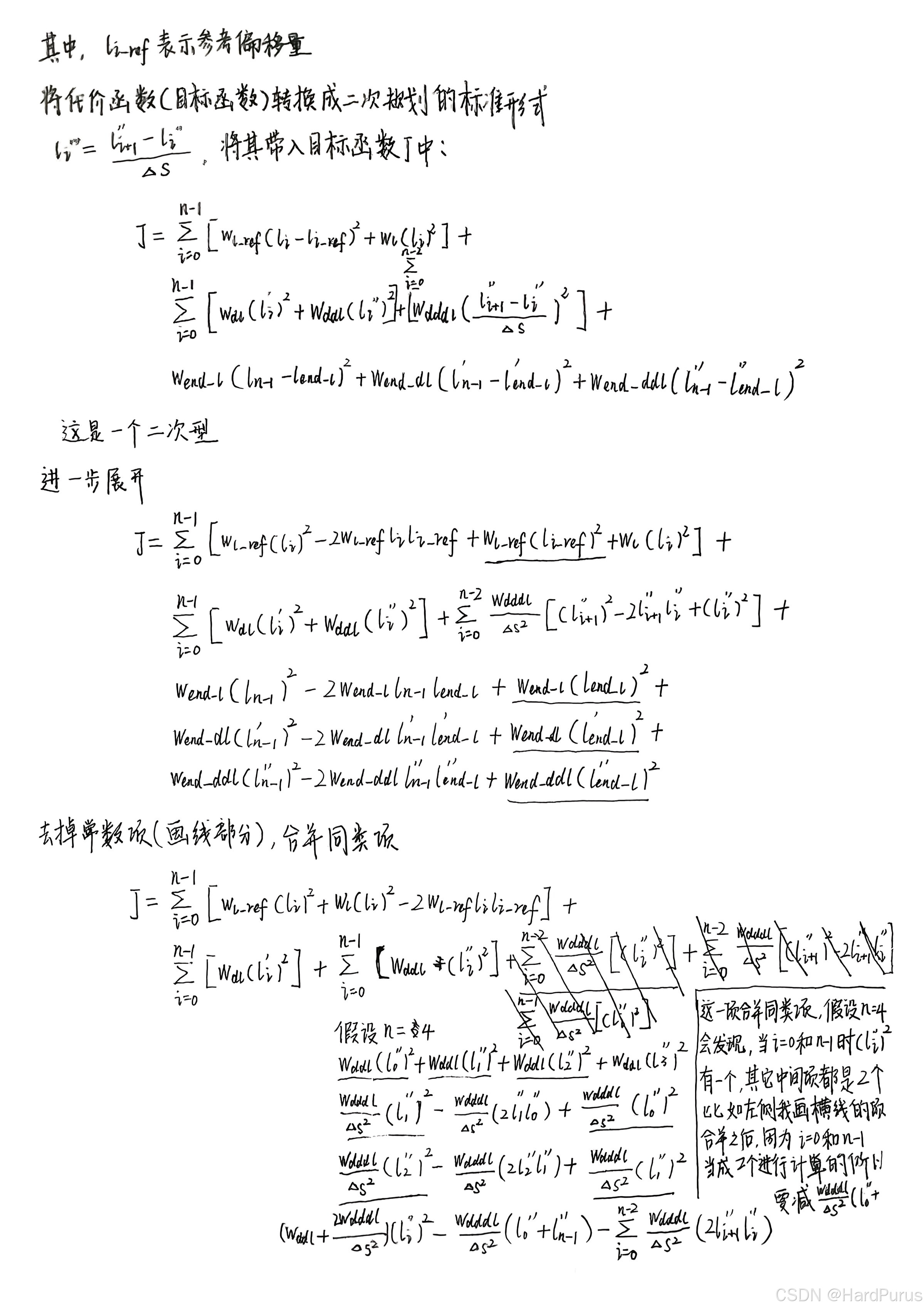
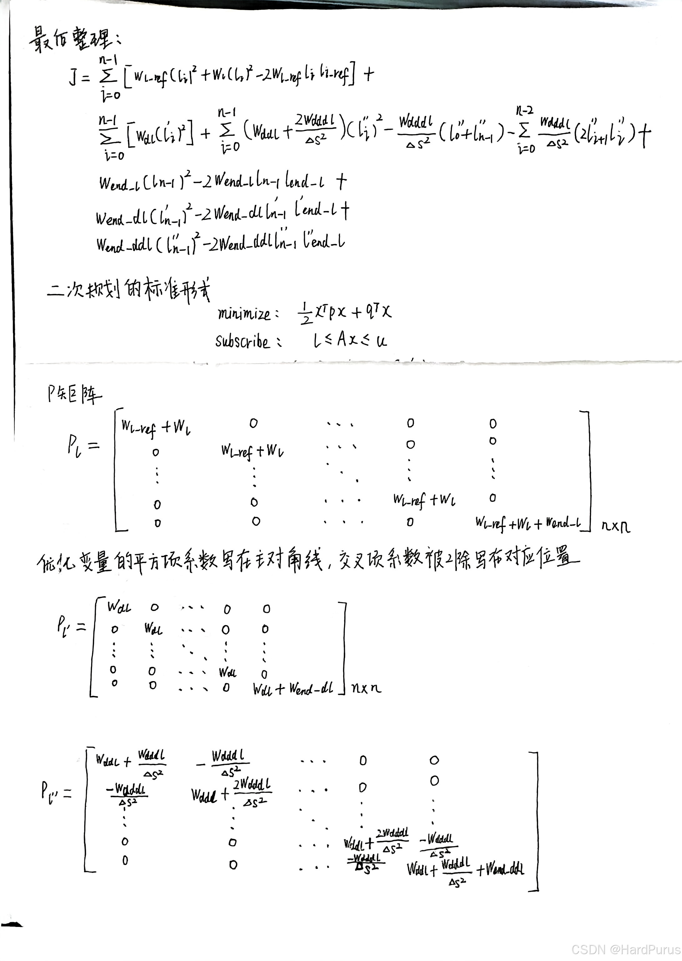
下面是假设n为4时的目标函数计算过程
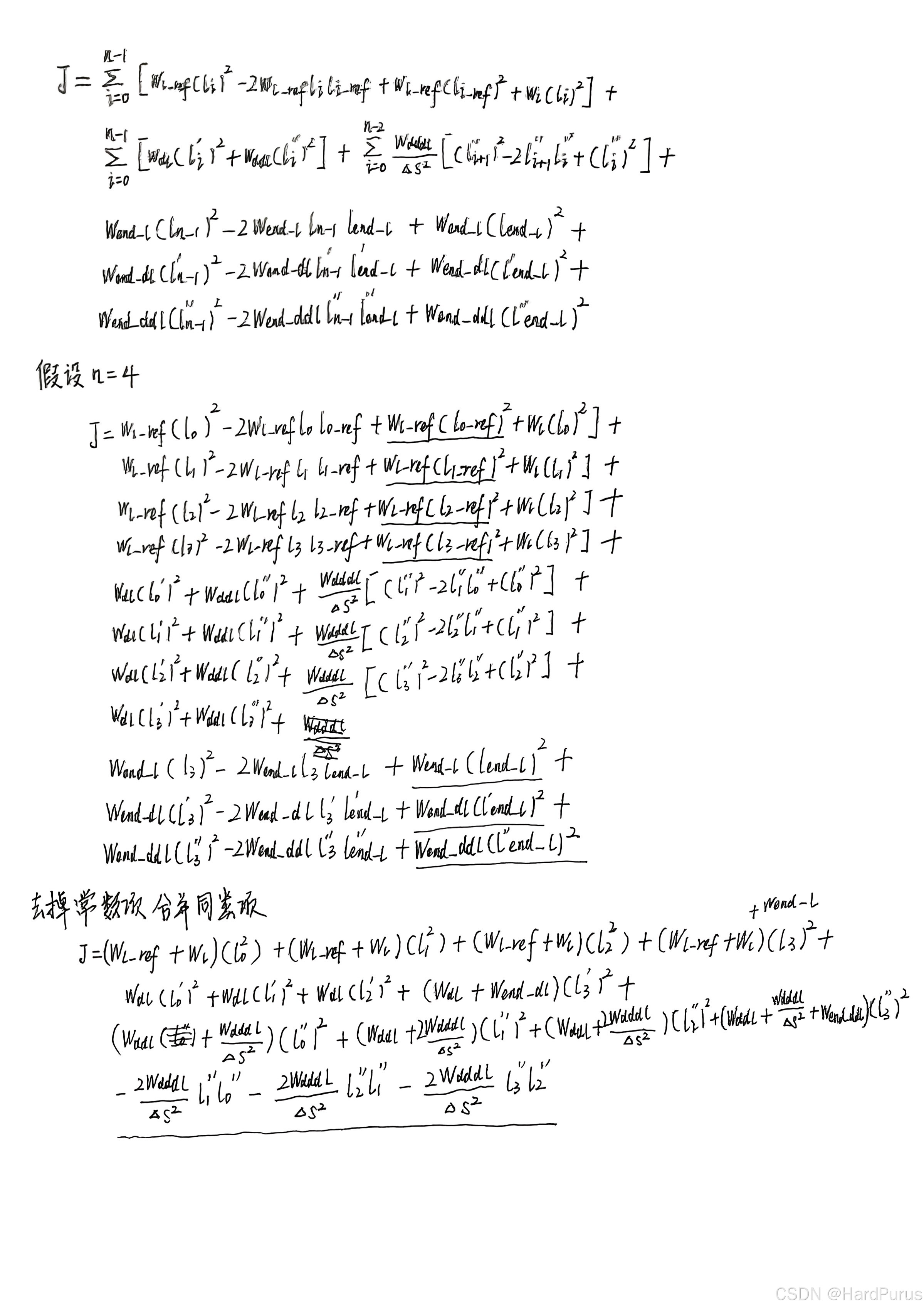
结合代码:
FormulateProblem函数
CalculateKernel函数
计算P矩阵
  for (int i = 0; i < n - 1; ++i) {
    columns[i].emplace_back(i, (weight_x_ + weight_x_ref_vec_[i]) /
                                   (scale_factor_[0] * scale_factor_[0]));
    ++value_index;
  }
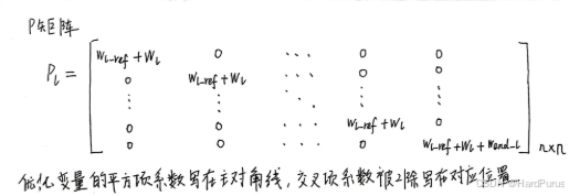
i \in [0,n-2]
columns[i][i]赋值为w_{l}+w_{l\_ref}
columns[n - 1].emplace_back(
      n - 1, (weight_x_ + weight_x_ref_vec_[n - 1] + weight_end_state_[0]) /
                 (scale_factor_[0] * scale_factor_[0]));
  ++value_index;
i = n - 1
columns[i][i]赋值为w_{l}+w_{l\_ref}+w_{end\_l}
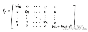
for (int i = 0; i < n - 1; ++i) {
    columns[n + i].emplace_back(
        n + i, weight_dx_ / (scale_factor_[1] * scale_factor_[1]));
    ++value_index;
  }
i \in [n,2n-2]
columns[i][i]:赋值为w_{dl}
i = 2n - 1;
columns[i][i]:赋值为w_{dl}+w_{end\_dl}
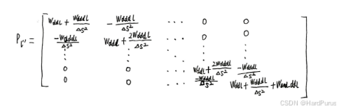
auto delta_s_square = delta_s_ * delta_s_;
  // x(i)''^2 * (w_ddx + 2 * w_dddx / delta_s^2)
  columns[2 * n].emplace_back(2 * n,
                              (weight_ddx_ + weight_dddx_ / delta_s_square) /
                                  (scale_factor_[2] * scale_factor_[2]));
i = 2n
columns[i][i]赋值为w\_ddl+ \frac{w\_{dddl}}{\Delta s^{2} }
  for (int i = 0; i < n - 1; ++i) {
    columns[2 * n + i + 1].emplace_back(
        2 * n + i, (-weight_dddx_ / delta_s_square) /
                        (scale_factor_[2] * scale_factor_[2]));
    ++value_index;
  }
i \in [2n + 1, 3n - 2]
columns[i][i - 1]赋值为\frac{-w\_{dddl}}{\Delta s^{2}}
++value_index;
  for (int i = 1; i < n - 1; ++i) {
    columns[2 * n + i].emplace_back(
        2 * n + i, (weight_ddx_ + 2.0 * weight_dddx_ / delta_s_square) /
                       (scale_factor_[2] * scale_factor_[2]));
    ++value_index;
  }
i \in [2n+1,3n-2]
columns[i][i]赋值为w\_{ddl}+\frac{2w\_{dddl}}{\Delta s^{2}}
columns[3 * n - 1].emplace_back(
      3 * n - 1,
      (weight_ddx_ + weight_dddx_ / delta_s_square + weight_end_state_[2]) /
          (scale_factor_[2] * scale_factor_[2]));
  ++value_index;
i = 3n - 1
columns[i][i]赋值为w\_{ddl}+\frac{w\_dddl}{\Delta s^{2}}+w\_{end\_ddl}
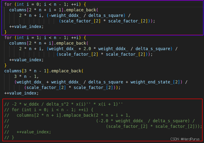
这里针对源代码对p矩阵的交叉项做了修改红色框注释掉的是原始逻辑,这是一个下三角,而osqp要求是上三角,并且交叉项的系数应该为\frac{-w\_dddl}{\Delta s^{2}}
根据上面假设n为4时的推导过程来看,交叉项的系数如上画线部分,而写成二次型矩阵形式的方法是,平方项系数写在主对角线,非平方项也就是交叉项系数被2除写在对应位置上,并且columns[col][row]是列行形式,比如-\frac{2w\_dddl}{\Delta s^{2}}l1''l0''的系数应该放在灰色交叉位置.
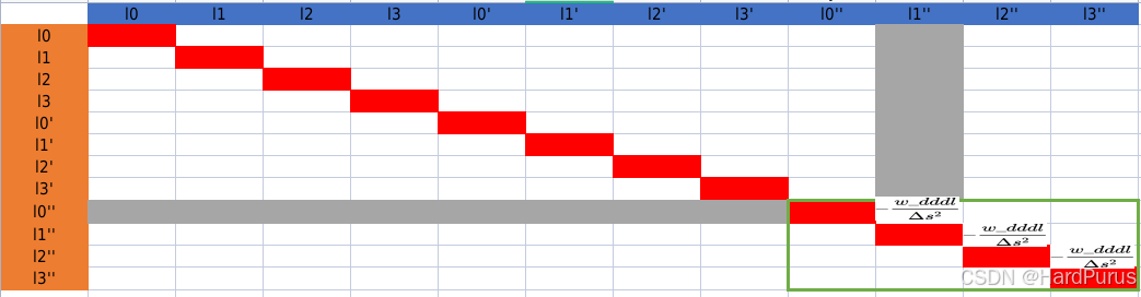
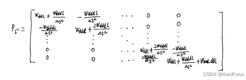
绿色框中是下方p_l^{''}的系数放置位置,只不过上图是n为4.
原始代码,由于写成了上三角导致目标函数对l'''的约束没有起作用,这样会导致自车横向出现跳变,导致即使路径边界范围足够,在转弯时也会转不过去,因为对l'''的约束没有起作用导致车辆在转弯时往参考线方向拉正的约束减小,而是往路沿方向上靠,导致转弯失败,修改后一般的弯道都是可以正常转过去的,效果很好.
  for (int i = 0; i < num_of_variables; ++i) {
    P_indptr->push_back(ind_p);
    for (const auto& row_data_pair : columns[i]) {
      P_data->push_back(row_data_pair.second * 2.0);
      P_indices->push_back(row_data_pair.first);
      ++ind_p;
    }
  }
上面逻辑依旧是CSC矩阵,可参考CSC(Compressed Sparse Column)矩阵
注意:columns[col][row]是按列行存储的
P_data:存储非0元素,按一列一列进行存储
P_indices:存储的是非0元素所在行
P_indptr:每一列非零元素在 P_data 的起始位置的索引
上面就是p矩阵的构建流程
CalculateAffineConstraint函数
计算A矩阵
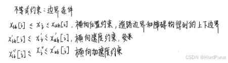
主要是二次规划中的约束条件
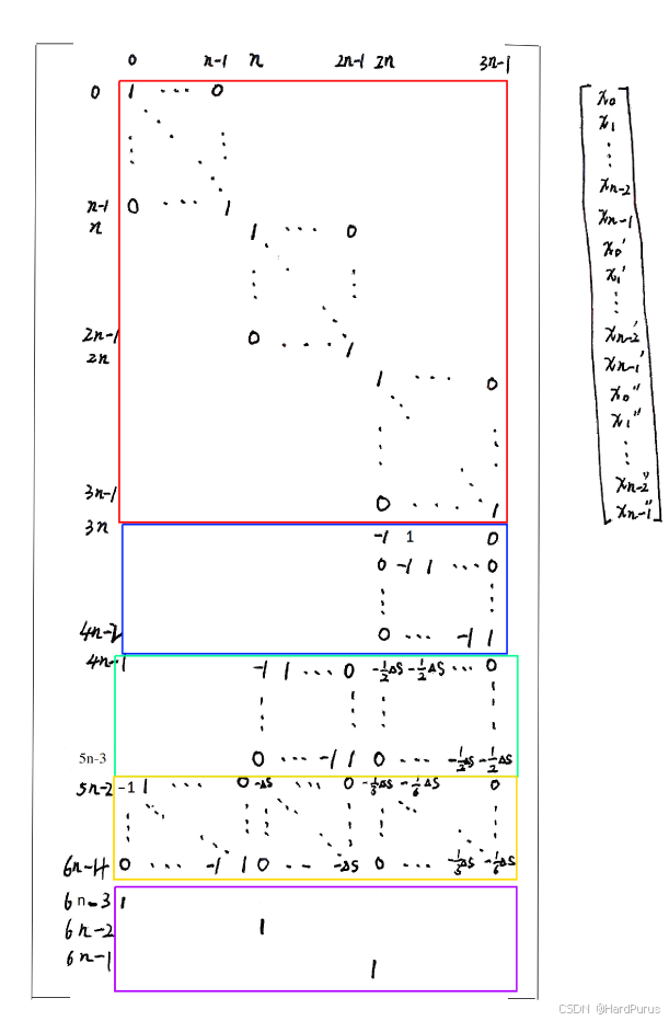
1.边界条件约束
for (int i = 0; i < num_of_variables; ++i) {
    if (i < n) {
      variables[i].emplace_back(constraint_index, 1.0);
      lower_bounds->at(constraint_index) =
          x_bounds_[i].first * scale_factor_[0];
      upper_bounds->at(constraint_index) =
          x_bounds_[i].second * scale_factor_[0];
    }
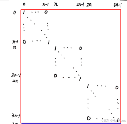
piecewise_jerk_problem.set_x_bounds(lat_boundaries);设置的所有路径点的路径边界
lower_bounds/upper_bounds:所有路径边界采样点的l约束范围
else if (i < 2 * n) {
      variables[i].emplace_back(constraint_index, 1.0);

      lower_bounds->at(constraint_index) =
          dx_bounds_[i - n].first * scale_factor_[1];
      upper_bounds->at(constraint_index) =
          dx_bounds_[i - n].second * scale_factor_[1];
    }
dx_bounds_:是通过函数piecewise_jerk_problem.set_dx_bounds(
-config.lateral_derivative_bound_default(),
config.lateral_derivative_bound_default());设置的对横向l'的约束范围,默认是\pm 2,从配置文件中获取到的
lower_bounds/upper_bounds:所有路径边界采样点的l'约束范围
else {
      variables[i].emplace_back(constraint_index, 1.0);
      lower_bounds->at(constraint_index) =
          ddx_bounds_[i - 2 * n].first * scale_factor_[2];
      upper_bounds->at(constraint_index) =
          ddx_bounds_[i - 2 * n].second * scale_factor_[2];
    }
ddx_bounds_:是通过函数piecewise_jerk_problem.set_ddx_bounds(ddl_bounds);设置的对横向l''的约束范围
这个范围是前面通过CalculateAccBound函数计算出来的
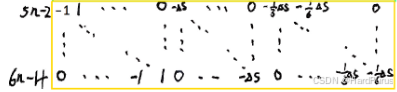
上面,三个逻辑的variables分别是上图中三个单位矩阵
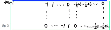
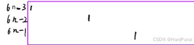
2.对l_{i}'''的约束
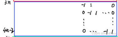
variables:系数如上
  for (int i = 0; i + 1 < n; ++i) {
    variables[2 * n + i].emplace_back(constraint_index, -1.0);
    variables[2 * n + i + 1].emplace_back(constraint_index, 1.0);
    lower_bounds->at(constraint_index) =
        dddx_bound_.first * delta_s_ * scale_factor_[2];
    upper_bounds->at(constraint_index) =
        dddx_bound_.second * delta_s_ * scale_factor_[2];
    ++constraint_index;
  }
lower_bounds/upper_bounds:是l_{i}'''要满足的范围
通过公式:
对两个点之间的加加速度(jerk)进行约束
dddx_bound_:是通过上面介绍的EstimateJerkBoundary函数获取到的
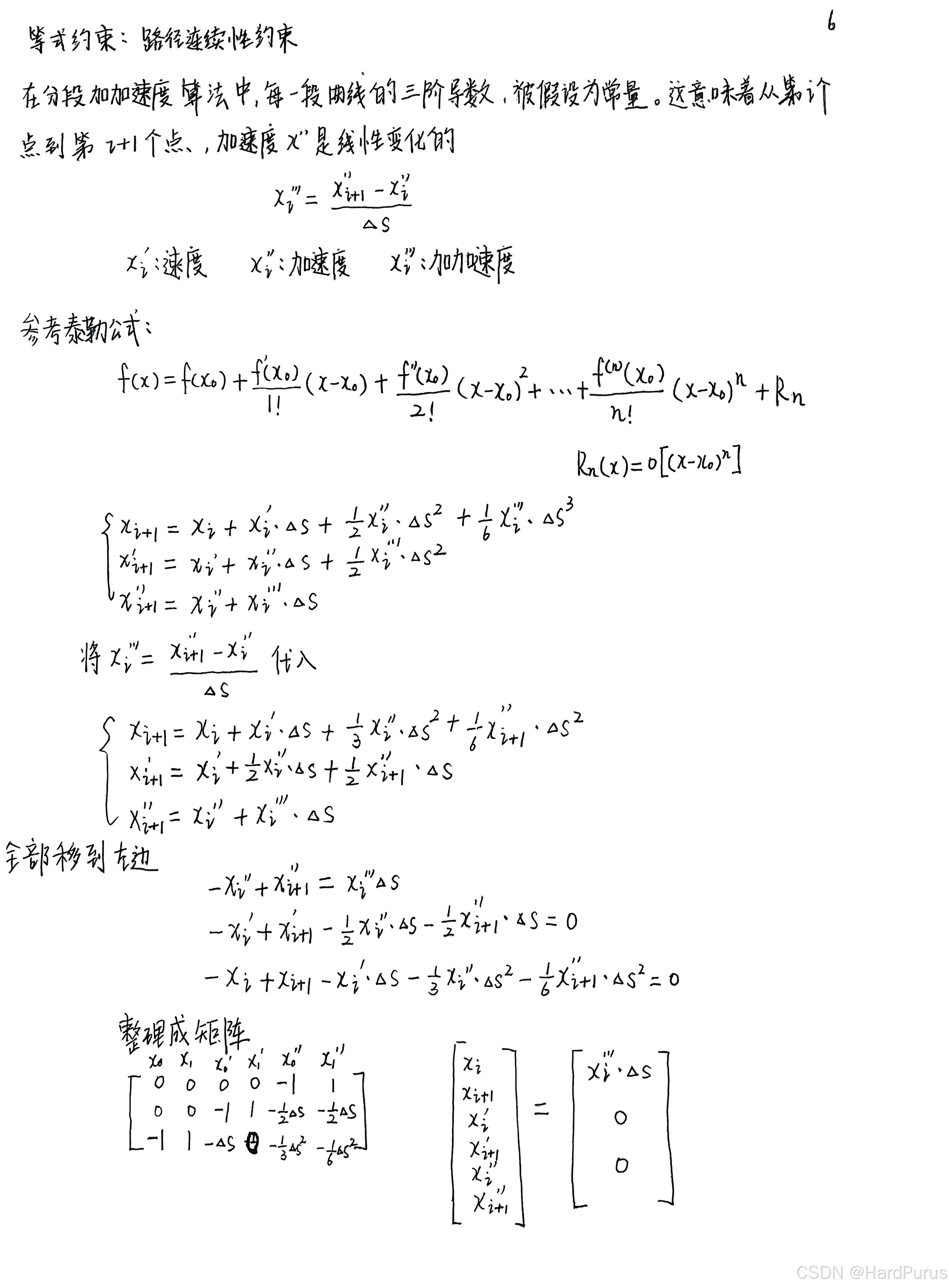
3.速度连续性约束
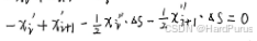
  for (int i = 0; i + 1 < n; ++i) {
    variables[n + i].emplace_back(constraint_index, -1.0 * scale_factor_[2]);
    variables[n + i + 1].emplace_back(constraint_index, 1.0 * scale_factor_[2]);
    variables[2 * n + i].emplace_back(constraint_index,
                                      -0.5 * delta_s_ * scale_factor_[1]);
    variables[2 * n + i + 1].emplace_back(constraint_index,
                                          -0.5 * delta_s_ * scale_factor_[1]);
    lower_bounds->at(constraint_index) = 0.0;
    upper_bounds->at(constraint_index) = 0.0;
    ++constraint_index;
  }
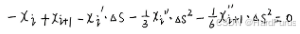
根据物理学的运动学公式,在一段位移 \Delta s 内,如果已知起点速度 x_i'、终点速度 x_{i+1}' 以及两点的加速度 x_i'', x_{i+1}'',我们可以用梯形积分法(中值定理的近似)来描述它们的关系:
整理成约束方程(右侧为 0)的形式:
系数矩阵
lower_bounds/upper_bounds:范围都设置为0
4.位置、加速度连续性约束
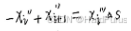
 auto delta_s_sq_ = delta_s_ * delta_s_;
  for (int i = 0; i + 1 < n; ++i) {
    variables[i].emplace_back(constraint_index,
                              -1.0 * scale_factor_[1] * scale_factor_[2]);
    variables[i + 1].emplace_back(constraint_index,
                                  1.0 * scale_factor_[1] * scale_factor_[2]);
    variables[n + i].emplace_back(
        constraint_index, -delta_s_ * scale_factor_[0] * scale_factor_[2]);
    variables[2 * n + i].emplace_back(
        constraint_index,
        -delta_s_sq_ / 3.0 * scale_factor_[0] * scale_factor_[1]);
    variables[2 * n + i + 1].emplace_back(
        constraint_index,
        -delta_s_sq_ / 6.0 * scale_factor_[0] * scale_factor_[1]);

    lower_bounds->at(constraint_index) = 0.0;
    upper_bounds->at(constraint_index) = 0.0;
    ++constraint_index;
  }
variables系数如下:
lower_bounds/upper_bounds:约束范围都设置为0
5.规划起点约束
  variables[0].emplace_back(constraint_index, 1.0);
  lower_bounds->at(constraint_index) = x_init_[0] * scale_factor_[0];
  upper_bounds->at(constraint_index) = x_init_[0] * scale_factor_[0];
  ++constraint_index;

  variables[n].emplace_back(constraint_index, 1.0);
  lower_bounds->at(constraint_index) = x_init_[1] * scale_factor_[1];
  upper_bounds->at(constraint_index) = x_init_[1] * scale_factor_[1];
  ++constraint_index;

  variables[2 * n].emplace_back(constraint_index, 1.0);
  lower_bounds->at(constraint_index) = x_init_[2] * scale_factor_[2];
  upper_bounds->at(constraint_index) = x_init_[2] * scale_factor_[2];
  ++constraint_index;
variables系数如下
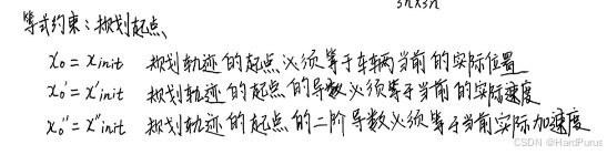
x_init_:是规划起点的{l, l', l''}
  int ind_p = 0;
  for (int i = 0; i < num_of_variables; ++i) {
    A_indptr->push_back(ind_p);
    for (const auto& variable_nz : variables[i]) {
      // coefficient
      A_data->push_back(variable_nz.second);

      // constraint index
      A_indices->push_back(variable_nz.first);
      ++ind_p;
    }
  }
  // We indeed need this line because of
  // https://github.com/oxfordcontrol/osqp/blob/master/src/cs.c#L255
  A_indptr->push_back(ind_p);
上面依旧是csc存储格式,上面已经介绍过了
CalculateOffset函数
计算q矩阵
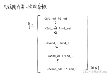
void PiecewiseJerkPathProblem::CalculateOffset(std::vector<c_float>* q) {
  CHECK_NOTNULL(q);
  const int n = static_cast<int>(num_of_knots_);
  const int kNumParam = 3 * n;
  q->resize(kNumParam, 0.0);

  if (has_x_ref_) {
    for (int i = 0; i < n; ++i) {
      q->at(i) += -2.0 * weight_x_ref_vec_.at(i) * x_ref_[i] / scale_factor_[0];
    }
  }

  if (has_end_state_ref_) {
    q->at(n - 1) +=
        -2.0 * weight_end_state_[0] * end_state_ref_[0] / scale_factor_[0];
    q->at(2 * n - 1) +=
        -2.0 * weight_end_state_[1] * end_state_ref_[1] / scale_factor_[1];
    q->at(3 * n - 1) +=
        -2.0 * weight_end_state_[2] * end_state_ref_[2] / scale_factor_[2];
  }
  if (has_towing_x_ref_) {
    for (int i = 0; i < n; ++i) {
      q->at(i) += -2.0 * weight_towing_x_ref_vec_.at(i) * towing_x_ref_[i] /
                  scale_factor_[0];
    }
  }
上面逻辑,先存疑我需要做一些仿真验证我的想法
这样FormulateProblem函数就介绍完了主要是介绍二次规划P,Q,A矩阵值的构造.
  osqp_work = osqp_setup(data, settings);
  osqp_solve(osqp_work);
然后通过osqp_solve函数进行二次规划问题的求解
  for (size_t i = 0; i < num_of_knots_; ++i) {
    x_.at(i) = osqp_work->solution->x[i] / scale_factor_[0];
    dx_.at(i) = osqp_work->solution->x[i + num_of_knots_] / scale_factor_[1];
    ddx_.at(i) =
        osqp_work->solution->x[i + 2 * num_of_knots_] / scale_factor_[2];
  }
求解出优化后的{l, l', l''},可以看出路径规划是横向优化
  *x = piecewise_jerk_problem.opt_x();
  *dx = piecewise_jerk_problem.opt_dx();
  *ddx = piecewise_jerk_problem.opt_ddx();
然后在modules/planning/planning_interface_base/task_base/common/path_util/path_optimizer_util.cc bool PathOptimizerUtil::OptimizePath函数中获取优化后的结果
到这PathOptimizerUtil::OptimizePath函数就介绍完了.