
本篇将介绍速度动态规划优化算法-path time heuristic optimizer(路径时间启发式优化器)
参考planning模块(9)-路径规划(scenario/stage/task) task的执行流程
for (auto task : task_list_) {
      const double start_timestamp = Clock::NowInSeconds();

      ret = task->Execute(frame, &reference_line_info);
modules/planning/planning_interface_base/task_base/common/speed_optimizer.cc
Status SpeedOptimizer::Execute(Frame* frame,
                               ReferenceLineInfo* reference_line_info) {
  Task::Execute(frame, reference_line_info);

  auto ret =
      Process(reference_line_info->path_data(), frame->PlanningStartPoint(),
              reference_line_info->mutable_speed_data());

  RecordDebugInfo(reference_line_info->speed_data());
  return ret;
}
modules/planning/tasks/path_time_heuristic/path_time_heuristic_optimizer.cc
Status PathTimeHeuristicOptimizer::Process(
    const PathData& path_data, const common::TrajectoryPoint& init_point,
    SpeedData* const speed_data)
path_data:是通过AssessPath函数获取到做过有效性检查的路径点数据
init_point:规划起点
path_data.discretized_path().empty()
DiscretizedPath::DiscretizedPath(std::vector<PathPoint> path_points)
    : std::vector<PathPoint>(std::move(path_points)) {}
是上一篇planning模块(12)-路径规划后构建速度规划所用的数据 路径点数据全部转化为笛卡尔坐标系下的数据的路径数据
SearchPathTimeGraph函数
const auto& dp_st_speed_optimizer_config =
      reference_line_info_->IsChangeLanePath()
          ? config_.lane_change_speed_config()
          : config_.default_speed_config();
变道和非变道使用不同的配置参数,配置文件路径:modules/planning/tasks/path_time_heuristic/conf/default_conf.pb.txt
GriddedPathTimeGraph函数
GriddedPathTimeGraph::GriddedPathTimeGraph(
    const StGraphData& st_graph_data, const DpStSpeedOptimizerConfig& dp_config,
    const std::vector<const Obstacle*>& obstacles,
    const common::TrajectoryPoint& init_point)
st_graph_data:存储ST图的所有数据
obstacles:所有障碍物
init_point:规划起点
DpStCost函数
DpStCost::DpStCost(const DpStSpeedOptimizerConfig& config, const double total_t,
                   const double total_s,
                   const std::vector<const Obstacle*>& obstacles,
                   const STDrivableBoundary& st_drivable_boundary,
                   const common::TrajectoryPoint& init_point)
config:速度动态规划优化器的配置
total_t:ST图上的总时间
total_s:ST图上的总纵向距离
st_drivable_boundary:ST可行驶区域边界,用于限制搜索空间
init_point:规划起点
for (const auto& obstacle : obstacles) {
  boundary_map_[obstacle->path_st_boundary().id()] = index++;
}
赋予障碍物ST边界的唯一ID
AddToKeepClearRange(obstacles);
AddToKeepClearRange函数
  for (const auto& obstacle : obstacles) {
    if (obstacle->path_st_boundary().IsEmpty()) {
      continue;
    }
    if (obstacle->path_st_boundary().boundary_type() !=
        STBoundary::BoundaryType::KEEP_CLEAR) {
      continue;
    }
    double start_s = obstacle->path_st_boundary().min_s();
    double end_s = obstacle->path_st_boundary().max_s();
    keep_clear_range_.emplace_back(start_s, end_s);
跳过没有ST边界的障碍物和边界类型不是禁停区的障碍物
当障碍物边界类型是禁停区时,获取障碍物ST边界纵向范围存入keep_clear_range_中
SortAndMergeRange(&keep_clear_range_);
void DpStCost::SortAndMergeRange(
    std::vector<std::pair<double, double>>* keep_clear_range) {
  if (!keep_clear_range || keep_clear_range->empty()) {
    return;
  }
  std::sort(keep_clear_range->begin(), keep_clear_range->end());
  size_t i = 0;
  size_t j = i + 1;
  while (j < keep_clear_range->size()) {
    if (keep_clear_range->at(i).second < keep_clear_range->at(j).first) {
      ++i;
      ++j;
    } else {
      keep_clear_range->at(i).second = std::max(keep_clear_range->at(i).second,
                                                keep_clear_range->at(j).second);
      ++j;
    }
  }
  keep_clear_range->resize(i + 1);
}
如果keep_clear_range中的相邻障碍物ST边界纵向范围存在重叠部分,就会对重叠部分进行合并
  const auto dimension_t =
      static_cast<uint32_t>(std::ceil(total_t / static_cast<double>(unit_t_))) +
      1;
计算时间维度,时间点的数量
  boundary_cost_.resize(obstacles_.size());
  for (auto& vec : boundary_cost_) {
    vec.resize(dimension_t, std::make_pair(-1.0, -1.0));
  }
  accel_cost_.fill(-1.0);
  jerk_cost_.fill(-1.0);
boundary_cost_:缓存每个障碍物在每个时间点的ST边界范围
accel_cost_:存储加速度成本
jerk_cost_:存储加加速度成本
到这DpStCost构造函数就介绍完了
total_length_t_ = st_graph_data_.total_time_by_conf();
total_length_t_:ST图在时间轴上的总长度,7s
unit_t_ = gridded_path_time_graph_config_.unit_t();
unit_t_:时间轴上每个网格的时间间隔,1s
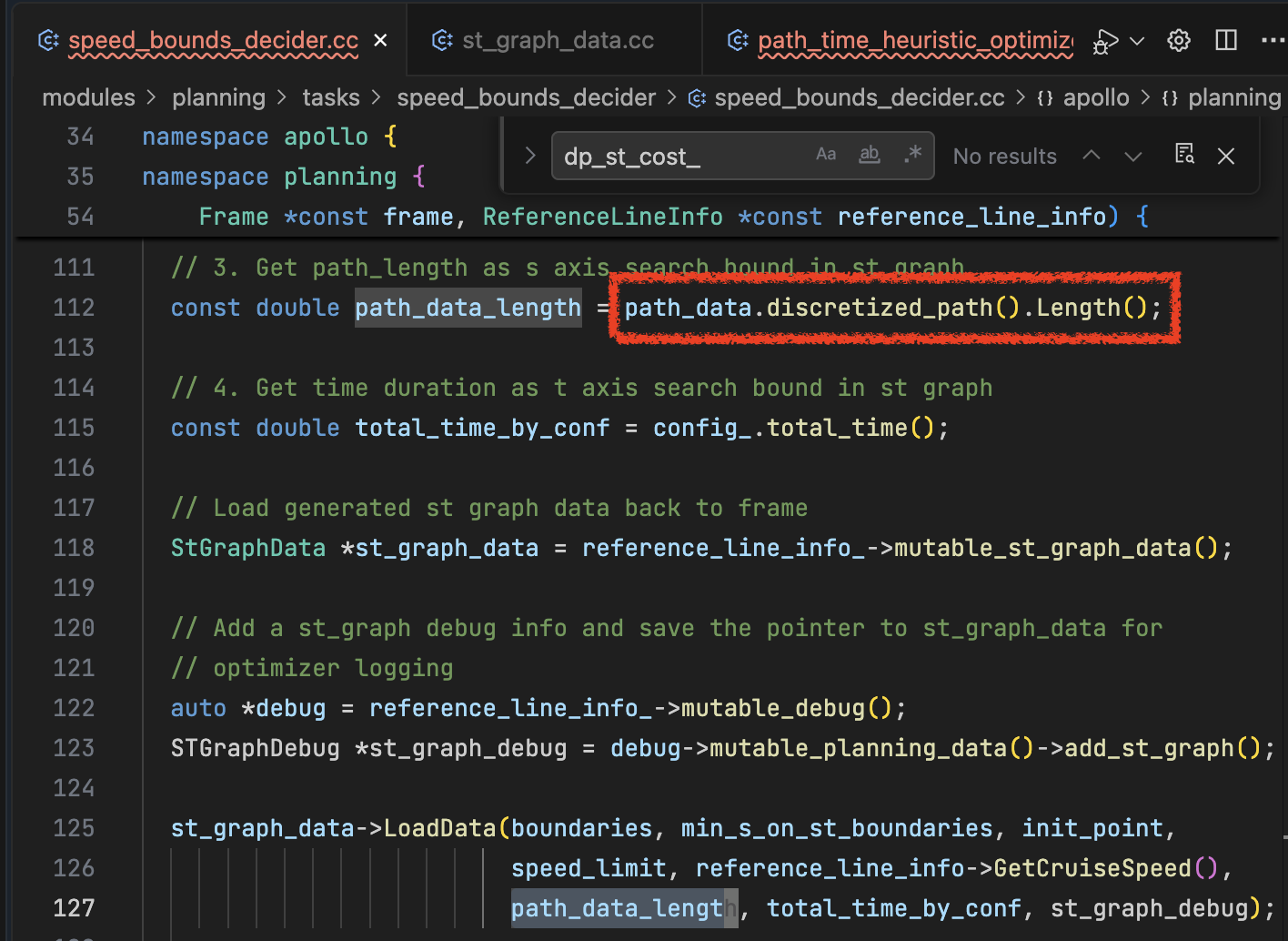
total_length_s_ = st_graph_data_.path_length();
参考线的总长度
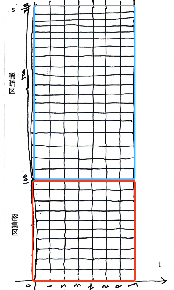
dense_unit_s_ = gridded_path_time_graph_config_.dense_unit_s();
dense_unit_s_:密集区域每个网格的纵向大小,车辆附近的轨迹需要高精度
巡航时配置:0.1m
换道时配置:0.25m
sparse_unit_s_ = gridded_path_time_graph_config_.sparse_unit_s();
sparse_unit_s_:稀疏区域每个网格的纵向大小,远距离规划不需要太高精度
巡航时配置:1.0m
换道时配置:1.0m
dense_dimension_s_ = gridded_path_time_graph_config_.dense_dimension_s();
dense_dimension_s_:纵向距离,密集区离散状态点的数量
巡航时配置:101个
换道时配置:21个
max_acceleration_ =
    std::min(std::abs(vehicle_param_.max_acceleration()),
             std::abs(gridded_path_time_graph_config_.max_acceleration()));
max_deceleration_ =
    -1.0 *
    std::min(std::abs(vehicle_param_.max_deceleration()),
             std::abs(gridded_path_time_graph_config_.max_deceleration()));
DP-ST图搜索中的加速度和减速度约束 ,确保规划出的速度轨迹符合车辆动力学特性和乘坐舒适性要求
max_acceleration_ =
     std::min(std::abs(vehicle_param_.max_acceleration()),
              std::abs(gridded_path_time_graph_config_.max_acceleration()));
 max_deceleration_ =
     -1.0 *
     std::min(std::abs(vehicle_param_.max_deceleration()),
              std::abs(gridded_path_time_graph_config_.max_deceleration()));
vehicle_param_.max_acceleration():车辆动力系统的最大加速能力,2m/s^2
gridded_path_time_graph_config_.max_acceleration():规划时采用的保守约束,2m/s^2
vehicle_param_.max_deceleration():车辆动力系统的最大减速能力,-6m/s^2
gridded_path_time_graph_config_.max_acceleration():规划时采用的保守约束,-4.0m/s^2
在车辆能力和规划约束之间选择更保守的值
到这GriddedPathTimeGraph函数就介绍完了
st_graph.Search(speed_data).ok()
调用动态规划算法在ST图上搜索最优路径,生成速度规划结果
Status GriddedPathTimeGraph::Search(SpeedData* const speed_data) {
for (const auto& boundary : st_graph_data_.st_boundaries()) {
    // KeepClear obstacles not considered in Dp St decision
    if (boundary->boundary_type() == STBoundary::BoundaryType::KEEP_CLEAR) {
      continue;
    }
遍历所有障碍物ST边界跳过ST边界类型是禁停区的障碍物
if (boundary->IsPointInBoundary({0.0, 0.0}) ||
      (std::fabs(boundary->min_t()) < kBounadryEpsilon &&
       std::fabs(boundary->min_s()) < kBounadryEpsilon))
IsPointInBoundary函数
bool STBoundary::IsPointInBoundary(const STPoint& st_point) const {
  if (st_point.t() <= min_t_ || st_point.t() >= max_t_) {
    return false;
  }
  size_t left = 0;
  size_t right = 0;
st_point:ST图的初始点(s=0.0, t=0.0)
IsPointInBoundary:检查点是否在障碍物ST边界内部
遍历所有障碍物的ST边界,然后判断ST图的初始点是否在障碍物的ST的边界内
GetIndexRange函数
bool STBoundary::GetIndexRange(const std::vector<STPoint>& points,
                               const double t, size_t* left,
                               size_t* right) const {
  CHECK_NOTNULL(left);
  CHECK_NOTNULL(right);
  if (t < points.front().t() || t > points.back().t()) {
    AERROR << "t is out of range. t = " << t;
    return false;
  }
points:是当前障碍物的ST边界的下边界点集
auto comp = [](const STPoint& p, const double t) { return p.t() < t; };
  auto first_ge = std::lower_bound(points.begin(), points.end(), t, comp);
  size_t index = std::distance(points.begin(), first_ge);
  if (index == 0) {
    *left = *right = 0;
  } else if (first_ge == points.end()) {
    *left = *right = points.size() - 1;
  } else {
    *left = index - 1;
    *right = index;
  }
在当前障碍物的ST边界的下边界点中,找到第一个大于等于ST图初始点时间的下边界点,然后获取到这个点在下边界点中的索引
如果索引index = 0,则让left = right = 0进行返回
如果在当前障碍物的ST边界的下边界中,没有找到大于等于ST图初始点时间的下边界点,则让 *left = *right = points.size() - 1进行返回
如果找到了第一个大于等于ST图初始点时间的下边界点,则令left = index - 1, right = index
right:是找到的第一个大于等于ST图初始点时间的下边界点的索引
left:是找到的这个下边界点的前一个点的索引
由于在apollo的代码里point_extension的配置默认是0,所以构建的障碍物的下边界和上边界的点集中S值都是正数
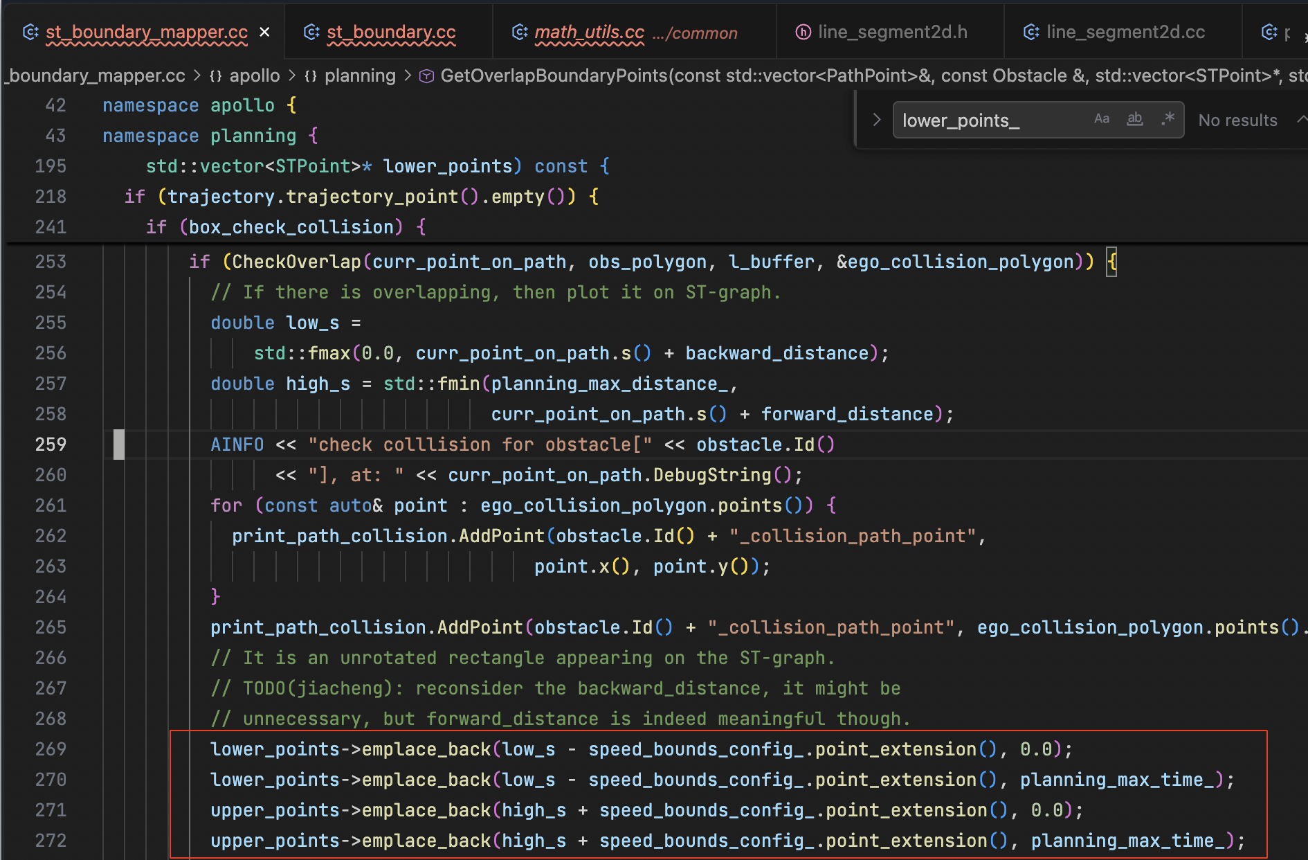
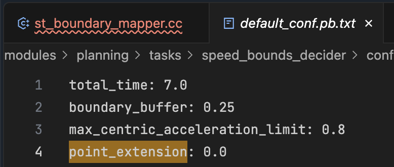
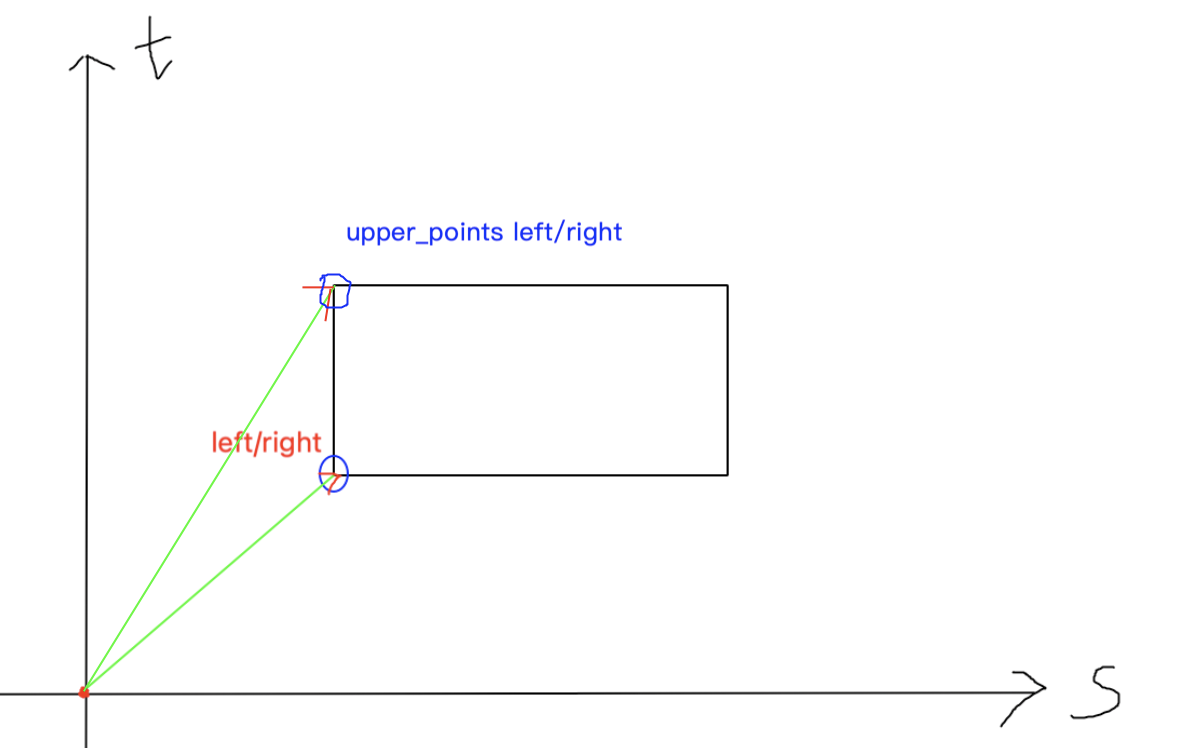
这就意味着ST图的初始点与从上边界点/下边界点获取到的left和right索引对应的边界点所构成的向量的叉积一直为0,也就意味着不会出现ST图初始点在障碍物ST边界范围内的情况
  const double check_upper = common::math::CrossProd(
      st_point, upper_points_[left], upper_points_[right]);
  const double check_lower = common::math::CrossProd(
      st_point, lower_points_[left], lower_points_[right]);

  return (check_upper * check_lower < 0);
也就意味着IsPointInBoundary函数不会返回true
可以先这么理解,如果在实际场景中发现理解错误再进行修改
std::fabs(boundary->min_t()) < kBounadryEpsilon &&
std::fabs(boundary->min_s()) < kBounadryEpsilon)
当障碍物中边界点中最小的纵向距离和时间很小时(ST初始点与障碍物很近时)
 dimension_t_ = static_cast<uint32_t>(std::ceil(
                    total_length_t_ / static_cast<double>(unit_t_))) +
                1;
 std::vector<SpeedPoint> speed_profile;
 double t = 0.0;
 for (uint32_t i = 0; i < dimension_t_; ++i, t += unit_t_) {
   speed_profile.push_back(PointFactory::ToSpeedPoint(0, t));
 }
 *speed_data = SpeedData(speed_profile);
unit_t_:是一个单位时间的步长,1.0s
total_length_t_:一次(一帧)规划的总时间,7.0s
dimension_t_:时间维度,时间索引点的数量,\left \lceil \frac{7}{1}+ 1\right \rceil=8
按照单位时间1.0s(也就是遍历的步长),遍历时间索引点的数量,初始化SpeedPoint结构
  static inline SpeedPoint ToSpeedPoint(const double s, const double t,
                                        const double v = 0, const double a = 0,
                                        const double da = 0) {
    SpeedPoint speed_point;
    speed_point.set_s(s);
    speed_point.set_t(t);
    speed_point.set_v(v);
    speed_point.set_a(a);
    speed_point.set_da(da);
    return speed_point;
  }
s:是纵向距离
t:是当前时间
v:是当前时间点的瞬时速率
a:当前时间加速度
da:当前时间的加加速度(jerk)
*speed_data = SpeedData(speed_profile);
构建参考线信息中的speed_data,作为障碍物与ST图初始点很近时的默认fallback轨迹速度规划数据
此时,速度,加速度,加加速度全都为0也就意味着车辆是停止状态
  if (!InitCostTable().ok()) {
    const std::string msg = "Initialize cost table failed.";
    AERROR << msg;
    return Status(ErrorCode::PLANNING_ERROR, msg);
  }
InitCostTable函数
巡航时
dense_dimension_s_:密集区纵向距离离散状态点的数量101
dense_dimension_s_ - 1:密集区网格数量,100
dense_unit_s_:密集区域网格单位长度0.1m
static_cast
 double sparse_length_s =
      total_length_s_ -
      static_cast<double>(dense_dimension_s_ - 1) * dense_unit_s_;
total_length_s_:路径规划出来的基于笛卡尔坐标系的离散后的规划路线长度
sparse_dimension_s_ =
 sparse_length_s > std::numeric_limits<double>::epsilon()
     ? static_cast<uint32_t>(std::ceil(sparse_length_s / sparse_unit_s_))
     : 0;
sparse_length_s:稀疏区域范围纵向距离长度
sparse_unit_s_:稀疏区域网格单位长度
sparse_dimension_s_ = std::ceil(sparse_length_s / sparse_unit_s_):稀疏区域网格数量
dimension_s_ = dense_dimension_s_ + sparse_dimension_s_;
dimension_s_:ST图表示纵向距离的网格数量
cost_table_ = std::vector<std::vector<StGraphPoint>>(
      dimension_t_, std::vector<StGraphPoint>(dimension_s_, StGraphPoint()));
构建dimension_t_行,dimension_s_列的cost_table_
 double curr_t = 0.0;
  for (uint32_t i = 0; i < cost_table_.size(); ++i, curr_t += unit_t_) {
    auto& cost_table_i = cost_table_[i];
    double curr_s = 0.0;
    for (uint32_t j = 0; j < dense_dimension_s_; ++j, curr_s += dense_unit_s_) {
      cost_table_i[j].Init(i, j, STPoint(curr_s, curr_t));
      debug.AddPoint("dp_node_points", curr_t, curr_s);
    }
初始化密集区ST图代价表
    curr_s = static_cast<double>(dense_dimension_s_ - 1) * dense_unit_s_ +
             sparse_unit_s_;
    for (uint32_t j = dense_dimension_s_; j < cost_table_i.size();
         ++j, curr_s += sparse_unit_s_) {
      cost_table_i[j].Init(i, j, STPoint(curr_s, curr_t));
      debug.AddPoint("dp_node_points", curr_t, curr_s);
    }
初始化稀疏区ST图代价表
  const auto& cost_table_0 = cost_table_[0];
  spatial_distance_by_index_ = std::vector<double>(cost_table_0.size(), 0.0);
  for (uint32_t i = 0; i < cost_table_0.size(); ++i) {
    spatial_distance_by_index_[i] = cost_table_0[i].point().s();
  }
spatial_distance_by_index_:行号到距离的映射数组
InitCostTable函数就介绍完了
InitSpeedLimitLookUp函数
 for (uint32_t i = 0; i < dimension_s_; ++i) {
    speed_limit_by_index_[i] =
        speed_limit.GetSpeedLimitByS(cost_table_[0][i].point().s());
  }
获取(0, s)位置的限速值
GetSpeedLimitByS函数
Status GriddedPathTimeGraph::InitSpeedLimitLookUp() {
  speed_limit_by_index_.clear();

  speed_limit_by_index_.resize(dimension_s_);
  const auto& speed_limit = st_graph_data_.speed_limit();
speed_limit:赋值可参考上一篇planning模块(14) task SPEED_BOUNDS_PRIORI_DECIDER LoadData函数
  for (uint32_t i = 0; i < dimension_s_; ++i)
    speed_limit_by_index_[i] =
        speed_limit.GetSpeedLimitByS(cost_table_[0][i].point().s());
  }
GetSpeedLimitByS函数
double SpeedLimit::GetSpeedLimitByS(const double s) const {
  CHECK_GE(speed_limit_points_.size(), 2U);
  DCHECK_GE(s, speed_limit_points_.front().first);

  auto compare_s = [](const std::pair<double, double>& point, const double s) {
    return point.first < s;
  };

  auto it_lower = std::lower_bound(speed_limit_points_.begin(),
                                   speed_limit_points_.end(), s, compare_s);

  if (it_lower == speed_limit_points_.end()) {
    return (it_lower - 1)->second;
  }
  return it_lower->second;
}
获取cost_table_代价表中(0, s)点的速度限制
CalculateTotalCost函数
CalculateTotalCost 第一性原理
本质问题
代码要解决什么物理问题?
自车从 (s=0, t=0) 出发,找一条最优的速度曲线。
怎么表示速度曲线?
在 ST 图上选一系列点:(0,0) → (c1,r1) → (c2,r2) → ... → (c_end, r_end)
什么叫最优?
这些点的 total_cost() 之和最小。
代码的本质(就一个公式)
// 第 429-440 行(c=2 的情况)
const double cost = cost_cr.obstacle_cost()
                  + cost_cr.spatial_potential_cost()
                  + pre_col[r_pre].total_cost()  // 前驱的成本
                  + CalculateEdgeCostForThirdCol(...);  // 从前驱走过来的成本

if (cost < cost_cr.total_cost()) {
  cost_cr.SetTotalCost(cost);  // 更新为更小的值
  cost_cr.SetPrePoint(pre_col[r_pre]);  // 记录从哪来
}
翻译成人话:
到当前点的成本 = 前驱的成本 + 从前驱走过来的成本

选哪个前驱?选让总成本最小的那个!
size_t next_highest_row = 0;
size_t next_lowest_row = 0;
[next_highest_row, next_lowest_row]:要遍历行数的范围
for (size_t c = 0; c < cost_table_.size(); ++c) {
最外层循环,遍历时间(T)维度
for (size_t r = next_lowest_row; r <= next_highest_row; ++r)
然后遍历纵向距离(S)维度
cost_table_代价表中时间维度表示列,距离维度表示行
for (size_t r = next_lowest_row; r <= next_highest_row; ++r) {
      const auto& cost_cr = cost_table_[c][r];
      if (cost_cr.total_cost() < std::numeric_limits<double>::infinity()) {
        size_t h_r = 0;
        size_t l_r = 0;
        GetRowRange(cost_cr, &h_r, &l_r);
        highest_row = std::max(highest_row, h_r);
        lowest_row = std::min(lowest_row, l_r);
      }
    }
next_highest_row = highest_row;
next_lowest_row = lowest_row;
每次遍历完纵向距离维度(行)后,重新获取下一次要遍历的纵向距离维度(行)的范围
动态规划完整推导流程
网格配置
时间维度(4 列):
- unit_t_ = 1.0 秒
- dimension_t_ = 4 列(t = 0, 1, 2, 3 秒)
- 列号:c = 0, 1, 2, 3
空间维度(3 行):
- unit_s_ = 3.0 米
- dimension_s_ = 3 行(r = 0, 1, 2)
- spatial_distance_by_index_ = [0.0, 3.0, 6.0] 米
初始状态:
- init_point_.v() = 3.0 m/s
- init_point_.a() = 0.0 m/s²
- init_point_.s() = 0.0 m
- init_point_.t() = 0.0 s
约束条件:
- max_acceleration_ = 1.5 m/s²
- max_deceleration_ = -1.5 m/s²
- FLAGS_planning_upper_speed_limit = 10.0 m/s
- kSpeedRangeBuffer = 0.20
- min_s_consider_speed = unit_s_ * 7 = 21.0 米
配置参数(简化):
- config_.default_speed_cost() = 1.0
- config_.accel_penalty() = 1.0
- config_.decel_penalty() = 1.0
- config_.positive_jerk_coeff() = 0.5
- config_.negative_jerk_coeff() = 0.5
- obstacle_cost = 0.0(无障碍)
- spatial_potential_cost = 0.0(简化)
- speed_cost = 0.0(假设速度合理,不超速也不低速)
- accel_cost = 1.0 * accel²(加速度平方,系数为 1)
- jerk_cost = 0.5 * jerk²(加加速度平方,系数为 0.5)
为了了解推导流程,简化代价计算
推导流程
初始化 cost_table_
所有点初始化为:
total_cost() = infinity
optimal_speed() = 0.0
pre_point() = nullptr
处理起点 (c=0, r=0)
调用:CalculateCostAt(msg={c: 0, r: 0})

c = 0, r = 0
cost_cr = cost_table_[0][0]

// 1. 初始化成本
cost_cr.SetObstacleCost(0.0)
cost_cr.SetSpatialPotentialCost(0.0)

// 2. c == 0,处理起点
cost_cr.SetTotalCost(0.0)
cost_cr.SetOptimalSpeed(init_point_.v()) = 3.0 m/s
return
结果
cost_table_[0][0]:
point: s=0.0m, t=0.0s
total_cost() = 0.0
optimal_speed() = 3.0 m/s
pre_point() = nullptr
处理第二列 (c=1)
计算 (c=1, r=0)
调用:CalculateCostAt(msg={c: 1, r: 0})

c = 1, r = 0
cost_cr = cost_table_[1][0]
cost_init = cost_table_[0][0]

// 1. 初始化成本
cost_cr.SetObstacleCost(0.0)
cost_cr.SetSpatialPotentialCost(0.0)

// 3. c == 1
// 计算加速度
point.s() = 0 * 3.0 = 0.0 米
acc = 2 * (0.0 / 1.0 - 3.0) / 1.0
    = 2 * (-3.0)
    = -6.0 m/s²

// 检查加速度约束
if (acc < max_deceleration_ || acc > max_acceleration_)
   (-6.0 < -1.5 || -6.0 > 1.5) ? 是!
→ return(减速度过大)
结果
cost_table_[1][0]:
total_cost() = infinity(不可达)
计算 (c=1, r=1)
调用:CalculateCostAt(msg={c: 1, r: 1})

c = 1, r = 1
cost_cr = cost_table_[1][1]
cost_init = cost_table_[0][0]

// 1. 初始化成本
cost_cr.SetObstacleCost(0.0)
cost_cr.SetSpatialPotentialCost(0.0)

// 3. c == 1
// 计算加速度
point.s() = 1 * 3.0 = 3.0 米
acc = 2 * (3.0 / 1.0 - 3.0) / 1.0
    = 2 * (3.0 - 3.0)
    = 0.0 m/s²

// 检查加速度约束
if (0.0 < -1.5 || 0.0 > 1.5) ? 否 ✓

// 检查速度
init_point_.v() + acc * unit_t_ = 3.0 + 0.0 * 1.0 = 3.0 m/s
if (3.0 < -kDoubleEpsilon && 3.0 > 21.0) ? 否 ✓

// 检查碰撞 ✓

// 计算总成本
// CalculateEdgeCostForSecondCol = speed_cost + accel_cost + jerk_cost
// speed_cost = 0.0(速度合理)
// accel_cost = 1.0 * accel² = 1.0 * 0.0² = 0.0
// jerk_cost = 0.5 * jerk² = 0.5 * 0.0² = 0.0

cost_cr.SetTotalCost(
    0.0 + 0.0 + cost_init.total_cost() + 0.0)
  = 0.0 + 0.0 + 0.0 + 0.0 = 0.0

cost_cr.SetPrePoint(cost_init) = cost_table_[0][0]
cost_cr.SetOptimalSpeed(init_point_.v() + acc * unit_t_)
  = 3.0 + 0.0 * 1.0 = 3.0 m/s
结果
cost_table_[1][1]:
point: s=3.0m, t=1.0s
total_cost() = 0.0
optimal_speed() = 3.0 m/s
pre_point() = cost_table_[0][0]
计算 (c=1, r=2)
调用:CalculateCostAt(msg={c: 1, r: 2})

c = 1, r = 2
cost_cr = cost_table_[1][2]

// 计算加速度
point.s() = 2 * 3.0 = 6.0 米
acc = 2 * (6.0 / 1.0 - 3.0) / 1.0
    = 2 * (6.0 - 3.0)
    = 6.0 m/s²

// 检查加速度约束
if (6.0 < -1.5 || 6.0 > 1.5) ? 是!
→ return(加速度过大)
结果
cost_table_[1][2]:
total_cost() = infinity(不可达)
处理第三列 (c=2)
计算 (c=2, r=0)
调用:CalculateCostAt(msg={c: 2, r: 0})

c = 2, r = 0
cost_cr = cost_table_[2][0]
point: s=0.0m, t=2.0s

// 1. 初始化成本
cost_cr.SetObstacleCost(0.0)
cost_cr.SetSpatialPotentialCost(0.0)

// 4. 计算搜索范围(详细步骤)
// 4.1 计算前一列的最低可达位置
// 物理含义:从当前点往回看,在 1 秒内以最大速度能到达的最远位置
pre_lowest_s = cost_cr.point().s() -
               FLAGS_planning_upper_speed_limit * (1 + kSpeedRangeBuffer) * unit_t_
             = 0.0 - 10.0 * (1 + 0.20) * 1.0
             = 0.0 - 12.0
             = -12.0 米

// 4.2 在 spatial_distance_by_index_ 中查找 >= pre_lowest_s 的最小位置
// spatial_distance_by_index_ = [0.0, 3.0, 6.0]
// 含义:每行对应的累积距离
pre_lowest_itr = std::lower_bound([0.0, 3.0, 6.0].begin(),
                                  [0.0, 3.0, 6.0].end(),
                                  -12.0)
               // lower_bound 返回第一个 >= -12.0 的迭代器
               // 0.0 >= -12.0,所以返回指向 0.0 的迭代器
               = 指向 [0.0] 的迭代器

// 4.3 计算 r_low(搜索范围的最小行号)
if (pre_lowest_itr == spatial_distance_by_index_.end()) {
  // 如果所有位置都 < pre_lowest_s,则 r_low = 最大行号
  r_low = dimension_s_ - 1 = 2
} else {
  // 否则计算迭代器的距离(索引)
  r_low = std::distance([0.0, 3.0, 6.0].begin(), 指向 [0.0] 的迭代器)
        = 0  // 第一个元素的索引是 0
}

// 4.4 计算搜索范围内的前驱点数量
// 当前行号 r = 0,搜索范围是 [r_low, r] = [0, 0]
r_pre_size = r - r_low + 1
           = 0 - 0 + 1
           = 1  // 只有 1 个前驱点需要检查

// 4.5 获取前一列的引用
pre_col = cost_table_[c - 1] = cost_table_[1]
// pre_col[0] = cost_table_[1][0]
// pre_col[1] = cost_table_[1][1]
// pre_col[2] = cost_table_[1][2]

// 4.6 初始化当前速度限制
curr_speed_limit = speed_limit = speed_limit_by_index_[0]

// 5. c == 2,遍历前驱(详细步骤)
// 循环次数:r_pre_size = 1
for (i = 0; i < 1; ++i) {
  // 5.1 计算前驱行号
  // i=0 时,r_pre = r - 0 = 0(检查第 0 行)
  // i=1 时,r_pre = r - 1(检查第 r-1 行)
  // 从当前行往下遍历,检查所有可能的前驱
  r_pre = r - i = 0 - 0 = 0

  // 5.2 检查前驱点是否可达
  // 条件 1:前驱点的 total_cost 不能是 infinity
  // 条件 2:前驱点必须有 pre_point(不是起点)
  if (std::isinf(pre_col[0].total_cost()) ||
      pre_col[0].pre_point() == nullptr) {
     // pre_col[0] = cost_table_[1][0]
     // cost_table_[1][0].total_cost() = infinity(之前计算的)
     // infinity == infinity ? 是!
     → continue(跳过这个前驱)
  }

  // 如果循环结束都没有找到合法前驱,则当前点也不可达
}

// 最终结果:没有合法前驱,cost_table_[2][0] 保持 infinity
结果
cost_table_[2][0]:
total_cost() = infinity(没有合法前驱)
计算 (c=2, r=1)
调用:CalculateCostAt(msg={c: 2, r: 1})

c = 2, r = 1
cost_cr = cost_table_[2][1]
point: s=3.0m, t=2.0s

// 1. 初始化成本
cost_cr.SetObstacleCost(0.0)
cost_cr.SetSpatialPotentialCost(0.0)

// 4. 计算搜索范围
// 4.1 计算 pre_lowest_s
pre_lowest_s = cost_cr.point().s() -
               FLAGS_planning_upper_speed_limit * (1 + kSpeedRangeBuffer) * unit_t_
             = 3.0 - 10.0 * 1.20 * 1.0
             = 3.0 - 12.0
             = -9.0 米

// 4.2 查找 r_low
pre_lowest_itr = std::lower_bound([0.0, 3.0, 6.0].begin(),
                                  [0.0, 3.0, 6.0].end(),
                                  -9.0)
               // 0.0 >= -9.0,返回指向 [0.0] 的迭代器
               = 指向 [0.0] 的迭代器

// 4.3 计算 r_low
r_low = std::distance([0.0, 3.0, 6.0].begin(), 指向 [0.0] 的迭代器)
      = 0

// 4.4 计算搜索范围大小
// 当前行号 r = 1,搜索范围是 [r_low, r] = [0, 1]
r_pre_size = r - r_low + 1
           = 1 - 0 + 1
           = 2  // 需要检查 2 个前驱点:r_pre = 1 和 r_pre = 0
                // - r_pre=1: cost_table_[1][1] (t=1.0s, s=3.0m)
                // - r_pre=0: cost_table_[1][0] (t=1.0s, s=0.0m)

// 4.5 获取前一列
pre_col = cost_table_[1]

// 4.6 初始化速度限制
curr_speed_limit = speed_limit_by_index_[1]

// 5. c == 2,遍历前驱
// 循环次数:r_pre_size = 2
for (i = 0; i < 2; ++i) {
  // ========== 第 1 次循环:i=0 ==========
  // 5.1 计算前驱行号
  r_pre = r - i = 1 - 0 = 1
  // 前驱点坐标:(t=1.0s, s=3.0m) ← cost_table_[1][1]

  // 5.2 检查前驱点是否可达
  if (std::isinf(pre_col[1].total_cost()) ||
      pre_col[1].pre_point() == nullptr) {
     // pre_col[1] = cost_table_[1][1]
     // cost_table_[1][1].total_cost() = 0.0 ✓
     // cost_table_[1][1].pre_point() = cost_table_[0][0] ✓
     → 条件不满足,继续执行
  }

  // 5.3 计算加速度
  // 公式:curr_a = 2 * ((当前 s - 前驱 s) / unit_t - 前驱速度) / unit_t
  curr_a = 2 * ((cost_cr.point().s() - pre_col[1].point().s()) / unit_t_ -
                pre_col[1].GetOptimalSpeed()) / unit_t_
         = 2 * ((3.0 - 3.0) / 1.0 - 3.0) / 1.0
         = 2 * (0.0 - 3.0)
         = 2 * (-3.0)
         = -6.0 m/s²

  // 5.4 检查加速度约束
  if (curr_a < max_deceleration_ || curr_a > max_acceleration_) {
     // -6.0 < -1.5 ? 是!
     → continue(减速度过大,跳过)
  }

  // ========== 第 2 次循环:i=1 ==========
  // 5.1 计算前驱行号
  r_pre = r - i = 1 - 1 = 0
  // 前驱点坐标:(t=1.0s, s=0.0m) ← cost_table_[1][0]

  // 5.2 检查前驱点是否可达
  if (std::isinf(pre_col[0].total_cost()) ||
      pre_col[0].pre_point() == nullptr) {
     // pre_col[0] = cost_table_[1][0]
     // cost_table_[1][0].total_cost() = infinity ✗
     → 条件满足,continue(跳过)
  }
}

// 最终结果:两个前驱都不合法,cost_table_[2][1] 保持 infinity
结果
cost_table_[2][1]:
total_cost() = infinity
计算 (c=2, r=2)
调用:CalculateCostAt(msg={c: 2, r: 2})

c = 2, r = 2
cost_cr = cost_table_[2][2]
point: s=6.0m, t=2.0s

// 1. 初始化成本
cost_cr.SetObstacleCost(0.0)
cost_cr.SetSpatialPotentialCost(0.0)

// 4. 计算搜索范围
// 4.1 计算 pre_lowest_s
pre_lowest_s = 6.0 - 10.0 * 1.20 * 1.0
             = 6.0 - 12.0
             = -6.0 米

// 4.2 查找 r_low
pre_lowest_itr = std::lower_bound([0.0, 3.0, 6.0].begin(),
                                  [0.0, 3.0, 6.0].end(),
                                  -6.0)
               // 0.0 >= -6.0,返回指向 [0.0] 的迭代器

// 4.3 计算 r_low
r_low = 0

// 4.4 计算搜索范围大小
// 当前行号 r = 2,搜索范围是 [r_low, r] = [0, 2]
//
// **为什么搜索范围是 [r_low, r] 而不是 [0, dimension_s_-1]?**
// 1. 上限是 r(当前行):
//    - 因为车辆不能"倒车",s 不能减小
//    - 前驱点的 s 必须 <= 当前点的 s
//    - 所以只需要检查行号 <= r 的点
//
// 2. 下限是 r_low:
//    - r_low 是根据 pre_lowest_s 计算出来的
//    - s < pre_lowest_s 的点,车辆无法在 1 秒内到达
//    - 这些点被剪枝掉,不需要检查
//
// 这就是为什么只检查"部分"前驱点,而不是所有点!
r_pre_size = r - r_low + 1
           = 2 - 0 + 1
           = 3  // 需要检查 3 个前驱点:r_pre = 2, 1, 0
                // - r_pre=2: cost_table_[1][2] (t=1.0s, s=6.0m)
                // - r_pre=1: cost_table_[1][1] (t=1.0s, s=3.0m)
                // - r_pre=0: cost_table_[1][0] (t=1.0s, s=0.0m)

// 4.5 获取前一列
pre_col = cost_table_[1]

// 4.6 初始化速度限制
curr_speed_limit = speed_limit_by_index_[2]

// 5. c == 2,遍历前驱
// 循环次数:r_pre_size = 3
for (i = 0; i < 3; ++i) {
  // ========== 第 1 次循环:i=0 ==========
  // 5.1 计算前驱行号
  r_pre = r - i = 2 - 0 = 2
  // 前驱点坐标:(t=1.0s, s=6.0m) ← cost_table_[1][2]

  // 5.2 检查前驱点是否可达
  if (std::isinf(pre_col[2].total_cost()) ||
      pre_col[2].pre_point() == nullptr) {
     // pre_col[2] = cost_table_[1][2]
     // cost_table_[1][2].total_cost() = infinity ✗
     → continue(跳过)
  }

  // ========== 第 2 次循环:i=1 ==========
  // 5.1 计算前驱行号
  r_pre = r - i = 2 - 1 = 1
  // 前驱点坐标:(t=1.0s, s=3.0m) ← cost_table_[1][1]

  // 5.2 检查前驱点是否可达
  if (std::isinf(pre_col[1].total_cost()) ||
      pre_col[1].pre_point() == nullptr) {
     // pre_col[1] = cost_table_[1][1]
     // cost_table_[1][1].total_cost() = 0.0 ✓
     // cost_table_[1][1].pre_point() = cost_table_[0][0] ✓
     → 条件不满足,继续执行
  }

  // 5.3 计算加速度
  curr_a = 2 * ((cost_cr.point().s() - pre_col[1].point().s()) / unit_t_ -
                pre_col[1].GetOptimalSpeed()) / unit_t_
         = 2 * ((6.0 - 3.0) / 1.0 - 3.0) / 1.0
         = 2 * (3.0 - 3.0)
         = 0.0 m/s²

  // 5.4 检查加速度约束
  if (curr_a < max_deceleration_ || curr_a > max_acceleration_) {
     // 0.0 < -1.5 ? 否
     // 0.0 > 1.5 ? 否
     → 条件不满足,继续执行
  }

  // 5.5 检查速度合理性
  if (pre_col[1].GetOptimalSpeed() + curr_a * unit_t_ < -kDoubleEpsilon &&
      cost_cr.point().s() > min_s_consider_speed) {
     // 3.0 + 0.0 * 1.0 = 3.0
     // 3.0 < -kDoubleEpsilon ? 否
     → 条件不满足,继续执行
  }

  // 5.6 检查碰撞
  if (CheckOverlapOnDpStGraph(st_graph_data_.st_boundaries(),
                              cost_cr, pre_col[1])) {
     // 假设无碰撞
     → 返回 false,继续执行
  }

  // 5.7 更新当前速度限制
  // 取当前行和前驱行的速度限制的最小值
  curr_speed_limit = std::fmin(curr_speed_limit,
                               speed_limit_by_index_[r_pre])
                   = std::fmin(speed_limit_by_index_[2],
                               speed_limit_by_index_[1])

  // 5.8 计算成本
  // CalculateEdgeCostForThirdCol = speed_cost + accel_cost + jerk_cost
  // first = cost_table_[0][0].point = (0.0, 0.0)
  // second = pre_col[1].point = (3.0, 1.0)
  // third = cost_cr.point = (6.0, 2.0)

  // speed_cost = 0.0(假设速度合理)
  // accel = (first.s + third.s - 2*second.s) / unit_t²
  //       = (0.0 + 6.0 - 2*3.0) / 1.0²
  //       = 0.0 m/s²
  // accel_cost = 1.0 * 0.0² = 0.0
  // jerk_cost = 0.0(c=2 时不计算 jerk)

  edge_cost = 0.0 + 0.0 + 0.0 = 0.0

  cost = cost_cr.obstacle_cost() +
         cost_cr.spatial_potential_cost() +
         pre_col[1].total_cost() +
         edge_cost
       = 0.0 + 0.0 + 0.0 + 0.0
       = 0.0

  // 5.9 更新最优解
  if (cost < cost_cr.total_cost()) {
     // 0.0 < infinity ? 是!
     cost_cr.SetTotalCost(0.0)
     cost_cr.SetPrePoint(pre_col[1])  // 记录前驱为 [1][1]
     cost_cr.SetOptimalSpeed(pre_col[1].GetOptimalSpeed() + curr_a * unit_t_)
       = 3.0 + 0.0 * 1.0 = 3.0 m/s
  }

  // ========== 第 3 次循环:i=2 ==========
  // 5.1 计算前驱行号
  r_pre = r - i = 2 - 2 = 0
  // 前驱点坐标:(t=1.0s, s=0.0m) ← cost_table_[1][0]

  // 5.2 检查前驱点是否可达
  if (std::isinf(pre_col[0].total_cost()) || ...) {
     // pre_col[0] = cost_table_[1][0]
     // cost_table_[1][0].total_cost() = infinity ✗
     → continue(跳过)
  }
}

// 最终结果:找到唯一合法前驱 [1][1],更新 cost_table_[2][2]
结果
cost_table_[2][2]:
point: s=6.0m, t=2.0s
total_cost() = 0.0
optimal_speed() = 3.0 m/s
pre_point() = cost_table_[1][1]
处理第四列 (c=3)
计算 (c=3, r=0)
调用:CalculateCostAt(msg={c: 3, r: 0})

c = 3, r = 0
cost_cr = cost_table_[3][0]
point: s=0.0m, t=3.0s

// 1. 初始化成本
cost_cr.SetObstacleCost(0.0)
cost_cr.SetSpatialPotentialCost(0.0)

// 4. 计算搜索范围
pre_lowest_s = 0.0 - 12.0 = -12.0
r_low = 0
r_pre_size = 0 - 0 + 1 = 1
pre_col = cost_table_[2]

// 遍历前驱 r_pre = 0
for (i = 0; i < 1; ++i) {
  r_pre = 0

  // 检查前驱点
  if (std::isinf(pre_col[0].total_cost()) || pre_col[0].pre_point() == nullptr)
     pre_col[0] = cost_table_[2][0]
     total_cost() = infinity ✗
  → continue
}
结果
cost_table_[3][0]:
 total_cost() = infinity
计算 (c=3, r=1)
调用:CalculateCostAt(msg={c: 3, r: 1})

c = 3, r = 1
cost_cr = cost_table_[3][1]
point: s=3.0m, t=3.0s

// 1. 初始化成本
cost_cr.SetObstacleCost(0.0)
cost_cr.SetSpatialPotentialCost(0.0)

// 4. 计算搜索范围
pre_lowest_s = 3.0 - 12.0 = -9.0
r_low = 0
r_pre_size = 1 - 0 + 1 = 2
pre_col = cost_table_[2]

// 遍历前驱 r_pre = 1, 0
for (i = 0; i < 2; ++i) {
  // i=0: r_pre = 1
  if (std::isinf(pre_col[1].total_cost()) || pre_col[1].pre_point() == nullptr)
     pre_col[1] = cost_table_[2][1]
     total_cost() = infinity ✗
  → continue

  // i=1: r_pre = 0
  if (std::isinf(pre_col[0].total_cost()) || ...)
     → continue
}
结果
cost_table_[3][1]:
 total_cost() = infinity
计算 (c=3, r=2)
调用:CalculateCostAt(msg={c: 3, r: 2})

c = 3, r = 2
cost_cr = cost_table_[3][2]
point: s=6.0m, t=3.0s

// 1. 初始化成本
cost_cr.SetObstacleCost(0.0)
cost_cr.SetSpatialPotentialCost(0.0)

// 4. 计算搜索范围
pre_lowest_s = 6.0 - 12.0 = -6.0
r_low = 0
r_pre_size = 2 - 0 + 1 = 3
pre_col = cost_table_[2]

// 遍历前驱 r_pre = 2, 1, 0
for (i = 0; i < 3; ++i) {
  // i=0: r_pre = 2
  if (std::isinf(pre_col[2].total_cost()) || pre_col[2].pre_point() == nullptr)
     pre_col[2] = cost_table_[2][2]
     total_cost() = 0.0 ✓
     pre_point() = cost_table_[1][1] ✓
  → 继续

  // 计算加速度
  curr_a = 2 * ((6.0 - 6.0) / 1.0 - 3.0) / 1.0
         = 2 * (0.0 - 3.0) = -6.0 m/s²
  if (-6.0 < -1.5) ? 是!→ continue

  // i=1: r_pre = 1
  if (std::isinf(pre_col[1].total_cost()) || ...)
     → continue

  // i=2: r_pre = 0
  if (std::isinf(pre_col[0].total_cost()) || ...)
     → continue
}
结果
cost_table_[3][2]:
total_cost() = infinity
cost_table_ 最终状态(4 列 × 3 行)
列号 c=0 (t=0.0s):
  [0][0]: total_cost=0.0, optimal_speed=3.0, pre_point=nullptr ✓
  [0][1]: 未处理
  [0][2]: 未处理

列号 c=1 (t=1.0s):
  [1][0]: total_cost=infinity (加速度 -6.0 过大) ✗
  [1][1]: total_cost=0.0, optimal_speed=3.0, pre_point=[0][0] ✓
  [1][2]: total_cost=infinity (加速度 6.0 过大) ✗

列号 c=2 (t=2.0s):
  [2][0]: total_cost=infinity (前驱 [1][0] 不可达) ✗
  [2][1]: total_cost=infinity (减速度 -6.0 过大) ✗
  [2][2]: total_cost=0.0, optimal_speed=3.0, pre_point=[1][1] ✓

列号 c=3 (t=3.0s):
  [3][0]: total_cost=infinity ✗
  [3][1]: total_cost=infinity ✗
  [3][2]: total_cost=infinity (减速度 -6.0 过大) ✗
唯一可达路径:
  (0,0) → (1,1) → (2,2)

成本累积:
  cost_table_[0][0] = 0.0
  cost_table_[1][1] = 0.0 + 0.0 = 0.0
  cost_table_[2][2] = 0.0 + 0.0 = 0.0

回溯:
  [2][2].pre_point() → [1][1]
  [1][1].pre_point() → [0][0]
  [0][0].pre_point() → nullptr
障碍物代价
double DpStCost::GetObstacleCost(const StGraphPoint& st_graph_point) {
  const double s = st_graph_point.point().s();
  const double t = st_graph_point.point().t();

  double cost = 0.0;
for (const auto* obstacle : obstacles_) {
auto boundary = obstacle->path_st_boundary();
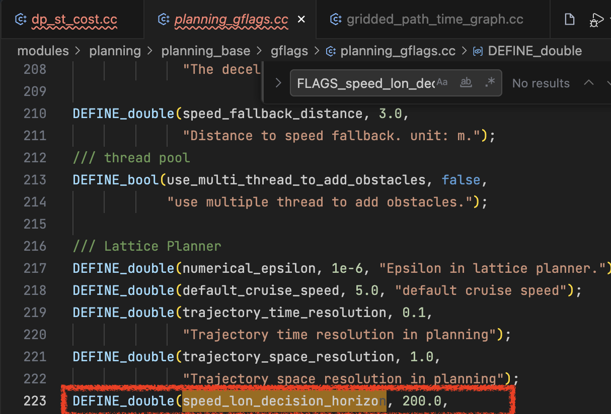
if (boundary.min_s() > FLAGS_speed_lon_decision_horizon) {
continue;
}
FLAGS_speed_lon_decision_horizon:纵向决策范围,默认是200m,如果障碍物不在纵向决策范围内,则忽略此障碍物
if (boundary.IsPointInBoundary(st_graph_point.point())) {
      return kInf;
    }
如果当前ST图中的点(s,t)在障碍物的ST边界范围内,就将该点的代价设置为无穷
int boundary_index = boundary_map_[boundary.id()];
 if (boundary_cost_[boundary_index][st_graph_point.index_t()].first < 0.0) {
   boundary.GetBoundarySRange(t, &s_upper, &s_lower);
   boundary_cost_[boundary_index][st_graph_point.index_t()] =
       std::make_pair(s_upper, s_lower);
 }
boundary_map_:可以理解为障碍物的ST边界id(障碍物id)与障碍物索引的对应关系
boundary_cost_:缓存每个障碍物在每个时间点的ST边界范围
if (boundary_cost_[boundary_index][st_graph_point.index_t()].first < 0.0) {
说明此时boundary_cost_[boundary_index][st_graph_point.index_t()]的边界范围还是初始值
GetBoundarySRange函数
用于查询指定时刻的 ST 边界纵向范围
bool STBoundary::GetBoundarySRange(const double curr_time, double* s_upper,
                                   double* s_lower) const {
  CHECK_NOTNULL(s_upper);
  CHECK_NOTNULL(s_lower);
  if (curr_time < min_t_ || curr_time > max_t_) {
    return false;
  }

  size_t left = 0;
  size_t right = 0;
  if (!GetIndexRange(lower_points_, curr_time, &left, &right)) {
    AERROR << "Fail to get index range.";
    return false;
  }
在障碍物下边界点集中,获取当前时间对应的索引范围
const double r =
(left == right
     ? 0.0
     : (curr_time - upper_points_[left].t()) /
           (upper_points_[right].t() - upper_points_[left].t()));
线性插值计算,当前ST图上的点所对应时间点在障碍物的ST边界上相对于right,left所对应的这段时间的比例
*s_upper = upper_points_[left].s() +
             r * (upper_points_[right].s() - upper_points_[left].s());
插值计算当前ST图上的点所对应时间点在障碍物的ST边界纵向边界上插值出来的上边界
*s_lower = lower_points_[left].s() +
             r * (lower_points_[right].s() - lower_points_[left].s());
插值计算当前ST图上的点所对应时间点在障碍物的ST边界纵向边界上插值出来的下边界
*s_upper = std::fmin(*s_upper, FLAGS_speed_lon_decision_horizon);
*s_lower = std::fmax(*s_lower, 0.0);
限制边界范围
到这GetBoundarySRange函数就介绍完了
boundary_cost_[boundary_index][st_graph_point.index_t()] =
          std::make_pair(s_upper, s_lower);
将获取到的通过障碍物ST纵向上下边界插值计算出的上下边界映射到ST图上对应的点上,这样就可以通过boundary_cost_根据时间查询障碍物的上下边界
else {
  s_upper = boundary_cost_[boundary_index][st_graph_point.index_t()].first;
  s_lower = boundary_cost_[boundary_index][st_graph_point.index_t()].second;
}
如果ST图上的某一个点,对应同一个障碍物,同一个时间点,则使用缓存中boundary_cost_已经计算好的上下边界,不再重新计算
if (s < s_lower) {
表示ST图上某个状态点的纵向距离值在障碍物后方
计算跟随成本
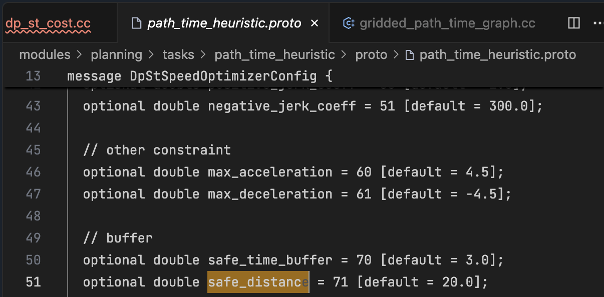
const double follow_distance_s = config_.safe_distance();
跟车安全距离默认是20m
if (s + follow_distance_s < s_lower) {
        continue;
      }
可以理解为当前这个ST图上的点的纵向距离加上跟车安全距离之后还是在障碍物后方,表示自车行驶到ST图这个时间点的时候不会和障碍物发生碰撞,所以不需要计算代价
else {
  auto s_diff = follow_distance_s - s_lower + s;
  cost += config_.obstacle_weight() * config_.default_obstacle_cost() *
          s_diff * s_diff;
}
使用距离差s_diff表示危险程度,使用距离差的二次函数计算障碍物成本
config_.default_obstacle_cost():障碍物成本的放大倍数,默认1e^{4}
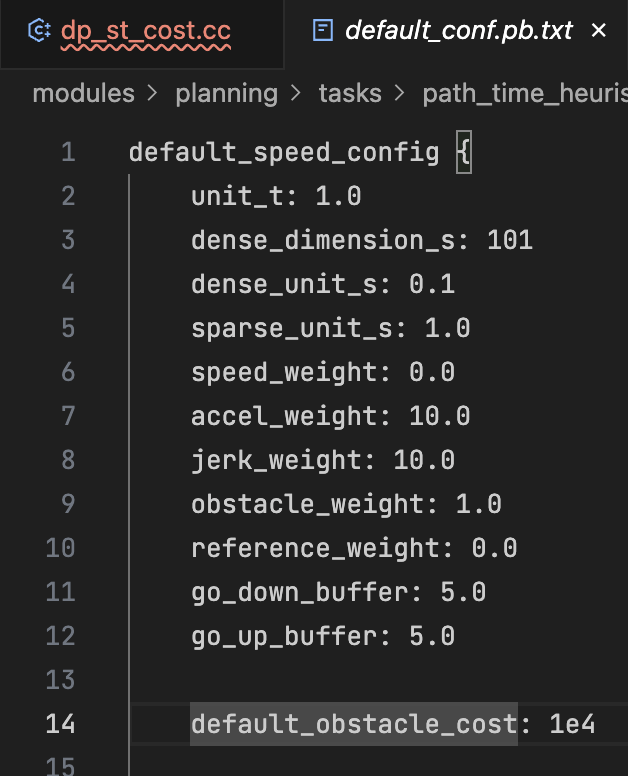
config_.obstacle_weight():是障碍物的权重系数,巡航时默认是1
ST图上点的障碍物成本代价,是与该点相关的障碍物的代价累加起来的总代价
else if (s > s_upper) {
表示ST图上某个状态点的纵向距离值在障碍物前方
计算超车成本
const double overtake_distance_s =
          StGapEstimator::EstimateSafeOvertakingGap();
安全超越距离
if (s > s_upper + overtake_distance_s) {  // or calculated from velocity
        continue;
      }
如果当前ST状态点的纵向距离大于安全超越所需的最小距离,表示该状态点不需要计算障碍物代价
else {
   auto s_diff = overtake_distance_s + s_upper - s;
   cost += config_.obstacle_weight() * config_.default_obstacle_cost() *
           s_diff * s_diff;
 }
如果当前ST状态点的纵向距离小于安全超越所需的最小距离,则同样使用距离差s_diff表示危险程度,使用距离差的二次函数计算障碍物成本,同样是所有相关障碍物代价累加起来的总代价
return cost * unit_t_;
其实本质上是
\int_{0}^{t} cost(t)dt
然后离散化,使用求和近似计算积分
\sum_{i = 0}^{t - 1} cost[i] \Delta t
(cost[0] + cost[1] + cost[2] + ... +cost[t-1])\Delta t
转换为代码就是cost * unit_t_
注意这里的cost * unit_t_只是上面(cost[0] + cost[1] + cost[2] + ... +cost[t-1])\Delta t代价中的一项障碍物代价
到这GetObstacleCost函数就介绍完了
  auto& cost_cr = cost_table_[c][r];

  cost_cr.SetObstacleCost(dp_st_cost_.GetObstacleCost(cost_cr));
  if (cost_cr.obstacle_cost() > std::numeric_limits<double>::max()) {
    return;
  }
然后将计算好的障碍物代价存储到cost_table_中,如果障碍物成本超过最大值(即无穷大),说明发生碰撞,直接返回
距离终点代价
GetSpatialPotentialCost函数
double DpStCost::GetSpatialPotentialCost(const StGraphPoint& point) {
  return (total_s_ - point.point().s()) * config_.spatial_potential_penalty();
}
距离路径规划终点越远代价越大,越近代价越小
total_s_:是笛卡尔坐标系下路径规划出来的轨迹长度
cost_cr.SetSpatialPotentialCost(dp_st_cost_.GetSpatialPotentialCost(cost_cr));
然后将计算好的距离终点代价存储到cost_table_中
CheckOverlapOnDpStGraph函数
检查从当前状态点到前驱状态点的直线路径是否与障碍物碰撞
bool CheckOverlapOnDpStGraph(const std::vector<const STBoundary*>& boundaries,
                             const StGraphPoint& p1, const StGraphPoint& p2) {
...
if (boundary->HasOverlap({p1.point(), p2.point()})) {
  return true;
}
bool Polygon2d::HasOverlap(const LineSegment2d &line_segment) const {
LineSegment2d::LineSegment2d(const Vec2d &start, const Vec2d &end)
    : start_(start), end_(end) {
  const double dx = end_.x() - start_.x();
  const double dy = end_.y() - start_.y();
  length_ = hypot(dx, dy);
  unit_direction_ =
      (length_ <= kMathEpsilon ? Vec2d(0, 0)
                               : Vec2d(dx / length_, dy / length_));
  heading_ = unit_direction_.Angle();
}
bool Polygon2d::HasOverlap(const LineSegment2d &line_segment) const {
  CHECK_GE(points_.size(), 3U);
  if ((line_segment.start().x() < min_x_ && line_segment.end().x() < min_x_) ||
      (line_segment.start().x() > max_x_ && line_segment.end().x() > max_x_) ||
      (line_segment.start().y() < min_y_ && line_segment.end().y() < min_y_) ||
      (line_segment.start().y() > max_y_ && line_segment.end().y() > max_y_)) {
    return false;
  }
这里先用线段和障碍物ST边界的笛卡尔坐标做了粗糙的碰撞检测
if (std::any_of(line_segments_.begin(), line_segments_.end(),
                  [&](const LineSegment2d &poly_seg) {
                    return poly_seg.HasIntersect(line_segment);
                  })) {
    return true;
  }
bool LineSegment2d::HasIntersect(const LineSegment2d &other_segment) const {
  Vec2d point;
  return GetIntersect(other_segment, &point);
}
GetIntersect函数
已经在planning模块(14) task SPEED_BOUNDS_PRIORI_DECIDER 介绍过了,可以回顾一下
 if (CheckOverlapOnDpStGraph(st_graph_data_.st_boundaries(), cost_cr,
                             cost_init)) {
   return;
 }
碰撞意味着这个状态点在物理上不可达,必须放弃,否则会选择危险的路径
    cost_cr.SetTotalCost(
        cost_cr.obstacle_cost() + cost_cr.spatial_potential_cost() +
        cost_init.total_cost() +
        CalculateEdgeCostForSecondCol(r, speed_limit, cruise_speed));
设置ST图当前状态点的总代价逻辑
当前状态点的总代价=障碍物代价+距离终点代价+前驱状态点总代价+边代价
边的代价
CalculateEdgeCostForSecondCol函数
计算初始状态点到第二列边的代价
double GriddedPathTimeGraph::CalculateEdgeCostForSecondCol(
    const uint32_t row, const double speed_limit, const double cruise_speed) {
  double init_speed = init_point_.v();
  double init_acc = init_point_.a();
  const STPoint& pre_point = cost_table_[0][0].point();
  const STPoint& curr_point = cost_table_[1][row].point();
  return dp_st_cost_.GetSpeedCost(pre_point, curr_point, speed_limit,
                                  cruise_speed) +
         dp_st_cost_.GetAccelCostByTwoPoints(init_speed, pre_point,
                                             curr_point) +
         dp_st_cost_.GetJerkCostByTwoPoints(init_speed, init_acc, pre_point,
                                            curr_point);
}
init_speed:初始状态点速度
init_acc:初始状态点加速度
pre_point:第二列的状态点的前驱都是初始状态点
curr_point:当前状态点
速度代价
GetSpeedCost函数
dp_st_cost_.GetSpeedCost(pre_point, curr_point, speed_limit,cruise_speed)
double DpStCost::GetSpeedCost(const STPoint& first, const STPoint& second,
                              const double speed_limit,
                              const double cruise_speed) const {
double cost = 0.0;
const double speed = (second.s() - first.s()) / unit_t_;
if (speed < 0) {
  return kInf;
}
计算平均速度,计算出的速度是负数,表示车辆在倒车直接返回无穷大代价
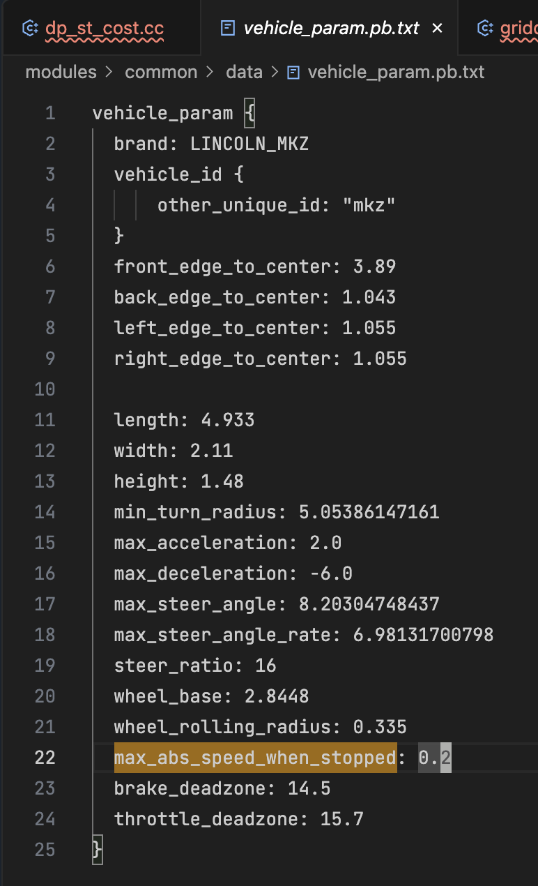
const double max_adc_stop_speed = common::VehicleConfigHelper::Instance()
                                        ->GetConfig()
                                        .vehicle_param()
                                        .max_abs_speed_when_stopped();
max_abs_speed_when_stopped:是一个速度阈值,默认是0.2m/s
- 速度 < 阈值 → 车辆视为"静止"
- 速度 ≥ 阈值 → 车辆视为"运动"
  if (speed < max_adc_stop_speed && InKeepClearRange(second.s())) {
    // first.s in range
    cost += config_.keep_clear_low_speed_penalty() * unit_t_ *
            config_.default_speed_cost();
  }
如果自车在禁停区并且接近停车状态时,施加惩罚
config_.keep_clear_low_speed_penalty():惩罚强度,默认为10
unit_t_:时间步长,默认1.0s
config_.default_speed_cost():代价基数,默认1.0e3
double det_speed = (speed - speed_limit) / speed_limit;
计算相对速度偏差
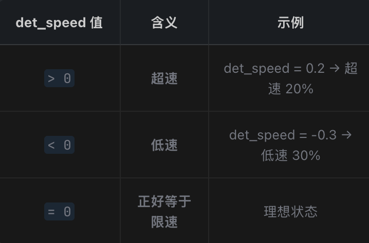
cost += config_.exceed_speed_penalty() * config_.default_speed_cost() *
            (det_speed * det_speed) * unit_t_;
超速惩罚代价 += 惩罚权重(1.0e3) * 代价基数(1.0e3) * (相对偏差)² * 时间步长
cost += config_.low_speed_penalty() * config_.default_speed_cost() *
            -det_speed * unit_t_
低速惩罚代价 += 惩罚权重(10.0) * 代价基数(1.0e3) * 相对偏差 * 时间步长
if (config_.enable_dp_reference_speed()) {
    double diff_speed = speed - cruise_speed;
    cost += config_.reference_speed_penalty() * config_.default_speed_cost() *
            fabs(diff_speed) * unit_t_;
  }
当启用参考速度功能时,惩罚偏离期望巡航速度的行为
加速度代价
GetAccelCostByTwoPoints函数
double DpStCost::GetAccelCostByTwoPoints(const double pre_speed,
                                         const STPoint& pre_point,
                                         const STPoint& curr_point) {
  double current_speed = (curr_point.s() - pre_point.s()) / unit_t_;
  double accel = (current_speed - pre_speed) / unit_t_;
计算当前加速度
\dot{s}=\frac{s_{1} - 0}{t_{1} - 0}
\ddot{s}=\frac{\dot{s} - 0}{t_{1} - 0}
GetAccelCost函数
 const double accel_sq = accel * accel;//加速度平方
 double max_acc = config_.max_acceleration();//最大加速度,2m/s^2
 double max_dec = config_.max_deceleration();//最大减速度, -4m/s^2
 double accel_penalty = config_.accel_penalty();//加速惩罚权重, 1.0
 double decel_penalty = config_.decel_penalty();//减速惩罚权重, 1.0
if (accel > 0.0) {
      cost = accel_penalty * accel_sq;
    } else {
      cost = decel_penalty * accel_sq;
    }
加速代价 = accel_penalty × accel²
减速代价 = decel_penalty × accel²
cost += accel_sq * decel_penalty * decel_penalty /
                (1 + std::exp(1.0 * (accel - max_dec))) +
            accel_sq * accel_penalty * accel_penalty /
                (1 + std::exp(-1.0 * (accel - max_acc)));
    accel_cost_.at(accel_key) = cost;
边界额外惩罚
到这GetAccelCost函数就介绍完了,GetAccelCostByTwoPoints函数也就介绍完了
GetJerkCostByTwoPoints函数
计算当前加加速度
\dot{s}=\frac{s_{1} - 0}{t_{1} - 0}
\ddot{s}=\frac{\dot{s} - \left | \vec{v} \right | }{t_{1} - 0}
\dddot{s}=\frac{\ddot{s} - \left | \vec{a} \right | }{t_{1} - 0}
const double curr_speed = (curr_point.s() - pre_point.s()) / unit_t_;
const double curr_accel = (curr_speed - pre_speed) / unit_t_;
const double jerk = (curr_accel - pre_acc) / unit_t_;
加加速度代价
JerkCost函数
if (jerk > 0) {
      cost = config_.positive_jerk_coeff() * jerk_sq * unit_t_;
    }
positive_jerk_coeff默认是1.0
cost = \omega_{pos} \cdot j^{2} \cdot \Delta t, j>0
else {
      cost = config_.negative_jerk_coeff() * jerk_sq * unit_t_;
    }
cost = \omega_{neg} \cdot j^{2} \cdot \Delta t, j>0
negative_jerk_coeff默认是1.0
return cost;
这里没有乘以unit_t_,因为在上面已经乘过了,为什么乘以unit_t_上面已经介绍过了
到这JerkCost函数就介绍完了,GetJerkCostByTwoPoints函数也介绍完了
return dp_st_cost_.GetSpeedCost(pre_point, curr_point, speed_limit,
                                  cruise_speed) +
         dp_st_cost_.GetAccelCostByTwoPoints(init_speed, pre_point,
                                             curr_point) +
         dp_st_cost_.GetJerkCostByTwoPoints(init_speed, init_acc, pre_point,
                                            curr_point);
最后得到边代价=速度代价+加速度代价+加加速度代价
到这CalculateEdgeCostForSecondCol函数就介绍完了
CalculateEdgeCost和CalculateEdgeCostForThirdCol的处理流程和CalculateEdgeCostForSecondCol差不多
RetrieveSpeedProfile函数
  for (const StGraphPoint& cur_point : cost_table_.back()) {
    if (!std::isinf(cur_point.total_cost()) &&
        cur_point.total_cost() < min_cost) {
      best_end_point = &cur_point;
      min_cost = cur_point.total_cost();
    }
  }
遍历最后一列的所有点
筛选可达点
找到成本最小的点作为最优终点
为后续的路径回溯提供起点
std::vector<SpeedPoint> speed_profile;
const StGraphPoint* cur_point = best_end_point;
PrintPoints debug_res("dp_result");
while (cur_point != nullptr) {
  ADEBUG << "Time: " << cur_point->point().t();
  ADEBUG << "S: " << cur_point->point().s();
  ADEBUG << "V: " << cur_point->GetOptimalSpeed();
  SpeedPoint speed_point;
  debug_res.AddPoint(cur_point->point().t(), cur_point->point().s());
  speed_point.set_s(cur_point->point().s());
  speed_point.set_t(cur_point->point().t());
  speed_profile.push_back(speed_point);
  cur_point = cur_point->pre_point();
}
- 路径回溯:从最优终点沿着pre_point()回到起点
- 生成速度曲线:将路径点转换为SpeedPoint格式
std::reverse(speed_profile.begin(), speed_profile.end());
将速度曲线反转,从"终点→起点"变为"起点→终点"的时间顺序
if (speed_profile.front().t() > kEpsilon ||
speed_profile.front().s() > kEpsilon) {
const std::string msg = "Fail to retrieve speed profile.";
AERROR << msg;
return Status(ErrorCode::PLANNING_ERROR, msg);
}
验证起点:确保速度曲线从原点(t=0, s=0)开始
for (size_t i = 0; i + 1 < speed_profile.size(); ++i) {
const double v = (speed_profile[i + 1].s() - speed_profile[i].s()) /
                 (speed_profile[i + 1].t() - speed_profile[i].t() + 1e-3);
speed_profile[i].set_v(v);
}

*speed_data = SpeedData(speed_profile);
计算每个速度点的速度值,并生成最终的速度数据对象,这里没有使用DP时的GetOptimalSpeed()速度,而是又通过差分重新计算了速度
到这reference_line_info->mutable_speed_data()的数据就计算完了